ABSTRACT
Determining the gradient of watercourses in the case of local applications is a common problem, which is most often dealt with by geodetic surveying. However, determining the gradient of all watercourses in the Czech Republic is a challenge. The use of geodetic methods on such a scale is usually unrealistic. Therefore, it is necessary to choose a different approach, such as the extraction of the gradient lines from other already existing elevation data. The DMR 4G and DMR 5G are elevation models currently available for the Czech Republic. For the extraction of gradient lines, it is necessary to create a digital terrain model (DTM) from the available datasets. Various interpolation methods are used for this. But which of the available interpolation methods is the most suitable? What role does the size of spatial resolution play in the quality of altimetry representation and subsequent sizes of the stored DTMs? To find answers to these questions, we chose four study sites (fourth order catchments) in the Otava river basin. Eight different DTMs were then created at each site, which were then compared. The results show that choice of raster size has a significantly greater influence on the resulting quality of the gradient lines than the choice of interpolation method in the case of DTM creation from DMR 5G data. DTM from DMR 4G data gives worse results than from DMR 5G at the same raster resolution.
INTRODUCTION
Determining the longitudinal slope of a watercourse bed is important from the point of view of a wide range of engineering and scientific applications, such as analysis of bed stability, detection of transverse obstacles, design of bed modification, and assessment of watercourse hydropower potential. In most cases, local studies requiring the slope of a watercourse bed use geodetic methods to survey them (tachymetry, positioning of GPS points). Geodetic approaches are very accurate; however, their use in the case of regional, district, or nationwide projects is not realistic. To survey an area the size of the Czech Republic, spatial data collection methods can be used. Satellite measurements or airborne laser scanning (ALS) methods are mainly used for this. Even today, satellites produce altimetry data with an error of several metres [1]. In contrast, ALS methods are able to achieve an error of only a few dozen cm [2, 3]. More recent studies report accuracy of a few cm [4]. Scanners with a beam with a wavelength close to the infrared spectrum are most often used for scanning the Earth’s surface. A specific feature of using infrared beams is the inability to measure under the water surface because water surface absorbs them. In such a location, the beam does not return to the measuring device, and thus does not determine the height mode. The advantage is a clear distinction between the water surface and the solid Earth surface [5]. However, there are variants of ALS that combine laser beams with different wavelengths (infrared and blue-green), which can also be used for scanning the terrain under the water surface [6].
The ALS method was used to survey the entire Czech Republic in 2009–2013. The measurement was carried out using LiteMapper 6800 device from IGI mbH using RIEGL LMS – Q680 aerial laser scanner. The measuring equipment was placed in a special L 410 FG aircraft. Scanning was done from an average height of 1,200 m or 1,400 m [7]. To scan the surface, RIEGL LMS – Q680 laser scanner uses a beam with a wavelength close to infrared spectrum [8]. The products of this focus are DMR 5G, DMR 4G and DMP 1G data sets. The first product available to users was DMR 4G data. The data can be found in the form of XYZ points at a regular spacing of 5 × 5 m. The height accuracy of this data is 0.3 m in open terrain and 1 m in densely built-up areas or forest cover. A certain limitation of this data layer may also be the reduced ability to describe fracture edges, which is based on the minimum spacing of points [9]. DMR 5G data is accessible in the form of irregularly spaced XYZ points. The height accuracy of this data is 0.18 m in open terrain and 0.3 m in densely built-up areas or forest cover. DMR 5G data is able to better describe terrain breaks and edges. Their disadvantage can be their volume, which is related to their point density [10]. DMP 1G data displays a digital model of the surface. This means that they also contain forest stands and buildings (listed in the real estate cadastre). However, in open terrain the data is identical to DMR 5G data [11].
It is usually not possible to compare directly the quality of the representation of the Earth’s surface with DMR 4G and DMR 5G data. The reason is a different position of source points in individual data sets. The solution to this problem is usually the use of interpolation methods, on the basis of which DMTs with identical resolution are created, which are then compared. Another possibility is the use of 3D control lines. Commonly used interpolation methods are Delaunay triangulation (TIN), inverse distances (IDW), minimum curvature (Spline), Natural Neighbor, or Kriging [12]. Evaluating the comparison of the interpolation method effect on the resulting quality of DMT based on DMR 5G data shows that different interpolation methods achieve comparable results both in open and in forested terrain. This is due to the high density of DMR 5G data [13].
MATERIAL AND METHODS
Study sites
Novosedelský stream – site No. 1
The site is located southwest of the town of Strakonice and is part of the Šumava foothills. From a morphological point of view, the area is located at altitudes ranging from 446.75 m to 864.131 m above sea level (a.s.l.), with a total height difference of 417.38 m a.s.l. The highest point of the area is in the south-eastern part and, conversely, the lowest point occurs in the north-eastern part of the site. The average altitude of the site is 636.386 m a.s.l.
Živný stream – site No. 2
The site is located southeast of the built-up area of the town of Prachatice and is also part of the Šumava foothills. The altitude ranges from 546.89 to 1,094.06 m a.s.l., with a total height difference of 547.17 m a.s.l. The highest point in the area is Libín hill in the eastern part of the site, and the lowest altitudes occur in the valley where the Živný potok flows. The average altitude of the site is 766.67 m a.s.l.
Širovská stoka – site No. 3
The site is located south of the town of Vodňany and is part of the České Budějovice Basin. From a morphological point of view, the site is located at altitudes ranging from 388.49 to 619.36 m a.s.l., with a total height difference of 230.86 m a.s.l. The highest point is Holička hill in the south-eastern part of the site. In contrast, the lowest point occurs in its northeastern part. The average altitude of the site is 451.23 m a.s.l.
Vydra – site No. 4
The site is located south of the village of Modrava, which is part of Šumava National Park. From a morphological point of view, it is located at altitudes ranging from 1,035.32 to 1,372.32 m a.s.l., with a total difference in height of 336.895 m a.s.l. The highest points of the area border the southern part of the study site and are formed by Blatný hill, Studená hora, Špičník, Hraniční hora, and Velká and Malá Mokrůvka. Towards the north of the area there is a significant decrease in altitude parallel to the Vydra riverbed. The average altitude of the site is 1,195.12 m a.s.l.
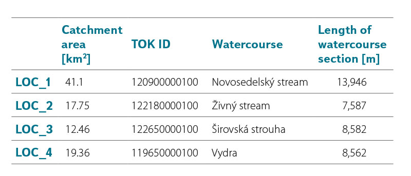
The overview of watercourses in the study sites is given in Tab. 1. The location of the study sites within the Czech Republic is shown in Fig. 1.
Tab. 1. Specifications of watercourses at study sites
 Obr. 1. Vybraná povodí IV. řádu a jejich lokalizace v rámci ČR. Barevně (oranžová, modrá, zelená, červená) jsou vyznačeny rozsahy (rozvodnice) jednotlivých povodí k příslušným vodním tokům. Stejnou barvou, jako mají rozvodnice, je pak vyznačena poloha daného povodí v rámci ČR. Tenká tmavě modrá linie ukazuje průběh vodních toků v rámci jejich povodí
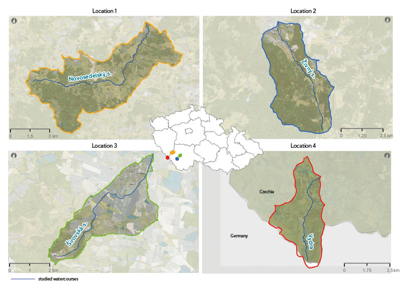
Fig. 1. Selected 4th order basins and their localization in the Czech Republic. The extents (watershed boundaries) of individual watersheds to the relevant watercourses are marked in color (orange, blue, green, red). The location of the watershed within the Czech Republic is marked with the same color as its watershed boundary. The thin dark blue line shows the position of the given watercourse in its catchment
Data description
When defining a suitable digital relief model (DMR) for determining the gradient on individual watercourses, two basic products of the Land Survey Office were used – the Digital Terrain Model of the Czech Republic of the 4th generation (DMR 4G) and the Digital Terrain Model of the Czech Republic of the 5th generation (DMR 5G) [7].
The fourth-generation digital terrain model of the Czech Republic represents the natural or human-modified Earth’s surface in digital form in via the heights of discrete points in a regular raster (5 × 5 m) of points with a complete mean height error of 0.3 m in open terrain and 1 m in forested terrain [9].
The fifth-generation digital terrain model of the Czech Republic represents natural or human-modified Earth surface in digital form via the heights of discrete points with a total mean height error of 0.18 m in open terrain and 0.3 m in forested terrain [10].
The watercourse axes for the study sites were taken from DIBAVOD (DIgitální BÁze VOdohospodářských Dat; Digital Database of Water Management Data). This is a water management extension of ZABAGED (Základní báze geografických dat; The Fundamental Base of Geographic Data of the Czech Republic). Specifically, layer A03 – watercourse (rough sections) was used, last updated on 5th June 2006. It is a section river model of main watercourses of fourth order catchments. The data is vector oriented in the direction of flow and provided in ESRI format [14].
All data used in this article were in the S-JTSK / Krovak East North coordinate system (EPSG 5514) and the Baltic height system after levelling (EPSG 5705).
METHODOLOGY
Creation of digital terrain models
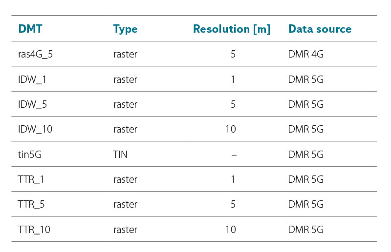
Terrain models were created in the ArcGIS Desktop environment. DMR 4G and DMR 5G datasets were used as input data for DMT creation. 8 DMTs were created for each site, i.e. 32 DMTs in total. The models can be divided into four groups based on the use of their data source and the interpolation method used for their creation. The first group of models was created from the DMR 4G dataset. Its representative is the ras4G_5 model. It is a raster model with a 5 × 5 m raster resolution produced by the Inverse Distance Weighting (IDW) method. The second group of models was also created using the IDW method, but from DMR 5G data. DMTs in this group differ from each other only in raster resolution. Three raster sizes of 1 m, 5 m and 10 m are used. The models are then labelled IDW_1, IDW_5 and IDW_10. The third group of models consists of tin5G. This is a TIN terrain model created from DMR 5G data. The fourth group of models is based on the TIN model from the third group, which was subsequently converted to rasters using the TinToRaster function. The models are labelled TTR_1, TTR_5 and TTR_10. They differ from each other only in the resulting raster size to which the models were transformed when they were converted from TIN format to raster format. A simple overview of DMT for each site and their specifications are given in Tab. 2.
Tab. 2. List of terrain models built for each study site
Extracting the 3D axis of watercourses
The 3D axes of the most important watercourses in the study sites (Fig. 1) were extracted from the prepared DMTs using the Interpolate Shape function. The identical Sampling Distance parameter was set for all extracted 3D line, which guaranteed that the height value on the watercourse line was always determined by the program for identical stationing. This is a basic condition for the possibility of comparing different height lines of one watercourse with each other. The 3D lines were exported to a text file using the Profile Graph function, where they were prepared for further comparison.
Evaluation of 3D lines
The actual processing was carried out in the R program. The 3D lines of the watercourse were loaded for individual sites and processed. DMT tin5G was always chosen as a reference for other raster DMTs of the given site. Mean Absolute Error (MAE) and Root Mean Square Error (RMSE) metrics were used to determine the degree of agreement.
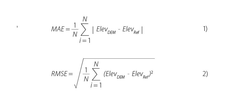
where:
ElevDEM is the elevation value (m) extracted from each DMT (ras4G_5, IDW_1, IDW_5, IDW_10, TTR_1, TTR_5, TTR_10)
ElevRef its corresponding elevation from the reference DMT (tin5G)
N number of height records on a given watercourse line
Comparison of DMT size when stored on Hard Disk Drive
In this comparison, the size of individual DMTs was determined when stored on a Hard Disk Drive (HDD). Subsequently, the relative sizes of the raster models compared to the comparative TIN models were calculated.
RESULTS
When comparing the quality of the height representation, it was found that the DMTs with a raster size of 1 m (DMT TTR_1 and IDW_1) showed the lowest mean errors. The worst results were achieved by DMTs with a raster size of 10 m (TTR_10, IDW_10), and the ras4G_5 model also achieved similarly poor results.
A visual comparison of the quality of the topographical description for selected watercourse sections in the Loc_4 site is shown in Fig. 2. In section U1, all DMTs show a similar quality of schematization. The only significantly different DMT is ras4G. In sections U2 and U3, a more significant deviation of the 10 m resolution models and the ras4G model can be seen.
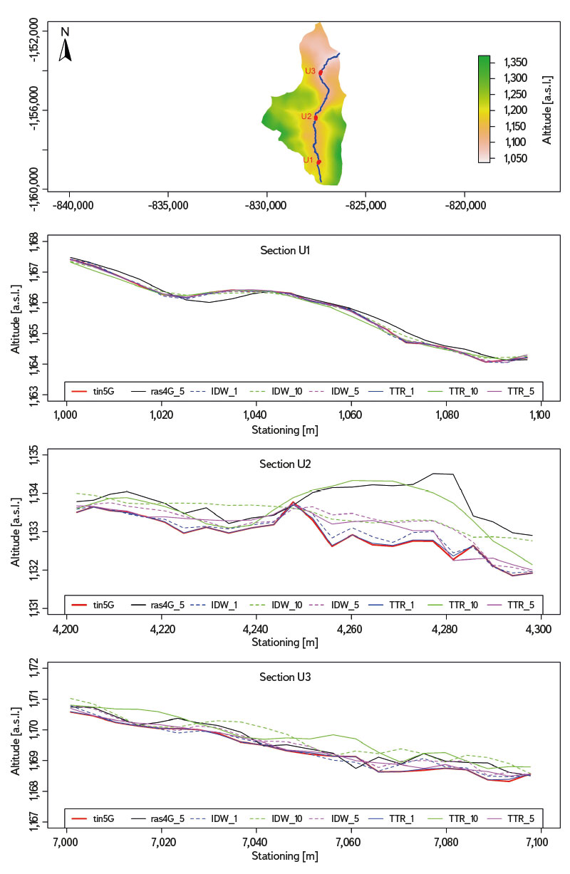
Fig. 2. Visual comparison of the quality of the slope lines extracted from the compared DTMs at the Loc_4 site
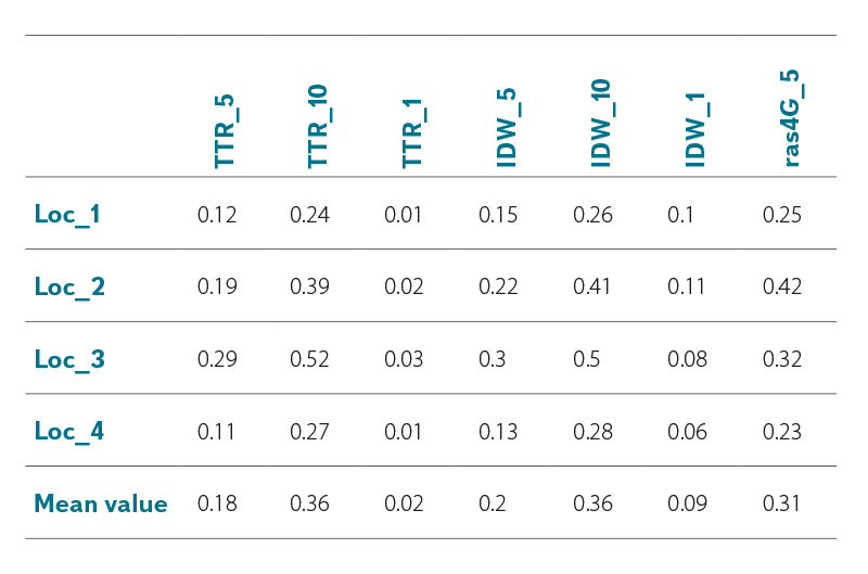
Models TTR_1 and IDW_1 showed the lowest mean absolute error (MAE). The mean error for TTR_1 was 0.02 m. The range of values ranged from 0.01 m (Loc_1 and Loc_4) to 0.03 m (Loc_3). IDW_1 achieved a mean error of 0.09 m with a range of 0.06 m (Loc_4) to 0.11 m (Loc_2). In contrast, the highest MAEs were found for the IDW_10 and TTR_10 models (both identically 0.36 m); with minimum values of 0.24 m. IDW_10 and TTR_10, they had almost identical error values even for the corresponding sites. The TTR_5 and IDW_5 models achieved an MAE of around 0.2 m. In contrast, the ras4G_5 model (same resolution) gave an error of 0.31 m. The overall overview of the MAE values is shown in Tab. 3.
Tab. 3. Summary of achieved MAE values
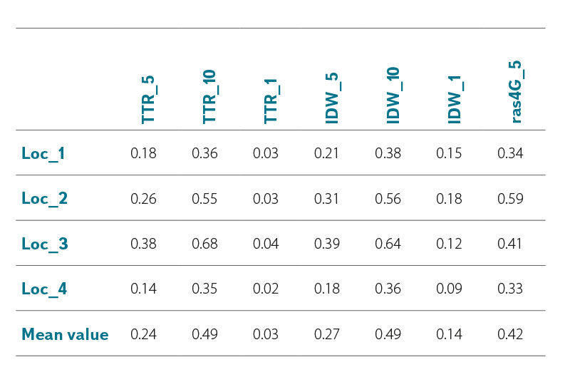
Also, the RMSE results show that the best values were achieved for the TTR_1 model, where the average RMSE error was 0.03 m. The worst results were again detected for the TTR_10 and IDW_10 models. Other values follow similar trends to the MAE values. The overall overview of RMSE values is shown in Tab. 4.
Tab. 4. Summary of achieved RMSE values
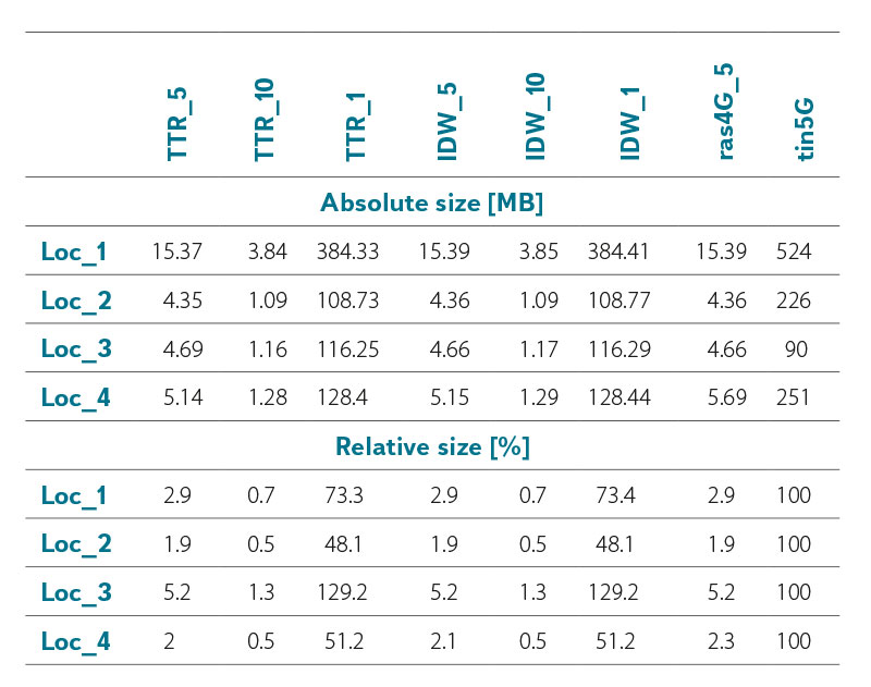
The physical size of individual DMTs when stored on a HDD was also evaluated. TIN models have the biggeststorage requirements. The only exception is at the site LOC_3, where the raster models with a resolution of 1 m are larger. The other DMTs with a 1 m raster have a size in the range of 50–75 %. The 5 m raster models have a consistent size ranging from 1.9–5.2 %. The 10 m raster models range within 0.5–1.3 %. The complete list of absolute and relative values of DMT sizes when saved to disk is shown in Tab. 5.
Tab. 5. Comparison of the amount of memory needed to store a given DTM on HDD
DISCUSSION
The tin5G model was chosen as the reference DMT. This model uses the maximum potential of the DMR 5G data set, i.e. all points and their absolute values for the creation of a complete digital terrain model. In contrast, raster models average the available point values within their raster. The fact that a large number of fourth order watercourses flow through the forested area also contributed to this choice. In such conditions, the TIN terrain model provides the best results [13].
There are multiple interpolation methods for creating DMT. In this paper, IDW methods and a combined DMT creation approach were used, when a TIN model was first created which was then transformed into a raster of the given size. The reason for choosing IDW and the combined approach was the speed of creating these terrain models in the R programming environment, which is planned to be used to process data for the entire Czech Republic. The fact that interpolation methods with high point density give the same results was also taken into account [13].
In the Czech Republic, in addition to DMR 4G and DMR 5G data, it is also possible to use 3D contours from the ZABAGED data layer to create DMT. These data were not included in the study; the decision was based on a literature search. The basis for ZABAGED 3D is the ZM 10 map from 1971–1988. These data are burdened by a greater degree of obsolescence (although some map sheets have been updated). Another disadvantage is systematic overestimation, which on average amounts to 0.23 m compared to DMR 5G data. The description using contours also touches on the issue of schematizing small terrain formations (small ridges and valleys) [15].
The results of this paper show the ability of individual DMTs to schematize the height of watercourses (thalwegs). The primary uncertainty of height schematization comes from the specifications of the source data [7, 9]. The authors are aware of these specifications. They are also aware of the limitations resulting from the ALS technology itself that was used for their acquisition (inability to scan watercourse beds). Another uncertainty is the quality of watercourse axis schematization in the DIBAVOD database, especially in forested terrain. In these places, the axis of the watercourse may be guided outside the actual watercourse bed. For the purpose of this study, it would be possible to create the watercourse axes manually; however, it is unrealistic for the application in the entire area of the Czech Republic.
When comparing MAEs, it can be tentatively concluded that raster models with a raster size of 1 m show better results than models with a larger raster size. The surprise was that the ras4G_5 model, which has a raster size of 5, gives similar results to models with a raster size of 10 (IDW_10, TTR_10). While maintaining this level of schematization quality, it would be worth considering whether to choose other models with a 10 m raster instead of the ras4G_5 model, which are also smaller (in terms of disk storage). This results in lower requirements for their computer processing. The best results were achieved by the TTR_1 model, which also outperformed the IDW_1 model. In this case, the method used to create the given terrain probably plays a role, especially the very principle of the IDW technique.
The RMSE values copy the MAE values to some extent. This is due to the fact that RMSE is based on MAE and is modified to reflect more the occurrence of extreme deviations [16]. In our case, it can therefore be stated that none of the tested DMTs carries extreme error values when compared.
A comparison of the physical size of individual rasters (i.e. the size they occupy on disk) shows how changing their spatial resolution (e.g. from 1 m to 5 m) dramatically reduces their size on disk. The exception is the IDW_1 and TTR_1 models at Loc_3. In this case, the size of the raster model exceeds the size of the TIN model, which may be caused by the flat nature of Loc_3. In the case of flat sites, DMR 5G provides a lower density of points than in sloping sites [10]. Lower point density reduces the size of the TIN model.
This article was created within the TA CR project TK04030223 and as such follows its goals. One of them is to create 3D lines of fourth order watercourses for the Czech Republic. For this purpose, it is necessary to use the available datasets covering the entire Czech Republic, process and evaluate them appropriately. Due to the scope of processing and evaluation, machine data processing is then necessary. It is also necessary to take into account the physical size of the produced DMTs due to their subsequent storage. Thus, this article is primarily intended to help answer the questions of which available data sets are the most suitable for the needs of the project and what spatial resolution of the rasters produced by DMT will be appropriate, especially with regard to their accuracy and storability.
CONCLUSION
The results of comparing the height schematization quality of the watercourse line, produced by different DMTs, show that models based on DMR 4G data achieve worse results than models with the same resolution based on DMR 5G data. When comparing models with the identical spatial resolution, based on DMR 5G data and created with a different interpolation method, it is evident that the choice of method for creating DMT plays a role, especially for rasters with a higher resolution. As resolution decreases, the importance of the interpolation method influence declines. The best MAE values were achieved by the TTR_1 model, with MAE of 0.02 m. The worst results were equally achieved by the TTR_10 and IDW_10 models, with MAE of 0.36 m. The RMSE values are only slightly different from the MAE values. It can therefore be assumed that none of the DMTs contain extreme values of residual errors.
Comparing the physical size of DMTs on disk shows how the size of raster DMTs increases with their resolution. The rasters with 1 m resolution reach 50–70 %, with 5 m 1.9–5.2 %, and with 10 m 0.5–1.3 % of the size of the corresponding TIN DMT. However, for rasters with a resolution of 1 m, this reduction does not always apply – it especially applies to flat basins, where the point density of DMR 5G data is low.
Acknowledgements
This article was created with the support of the Technology Agency of the Czech Republic as part of the project No. TK04030223 “Determination of hydropower potential of Pico-Hydropower in current and predicted climatic conditions of the Czech Republic”.
The Czech version of this article was peer-reviewed, the English version was translated from the Czech original by Environmental Translation Ltd.
