ABSTRACT
A wetland is an environment where water is readily available for vegetation, and therefore intensive evapotranspiration (ET) close to the potential ET value occurs. In addition, higher ET intensities can be expected in the future due to the observed increase in temperatures associated with climate change. The impact of wetland ET needs to be considered, for example, in restoration planning or hydrological modelling, and it is important to draw on the current knowledge provided by the large number of papers worldwide. Therefore, the first part of the paper is a brief review of existing research on wetland ET. The second part of the paper is a practical demonstration of the impact of ET on wetlands in the western part of the Bohemian Cretaceous Basin.
In the first (review) part of the paper, the articles were divided into several groups according to whether they were based on investigations of groundwater level (GWL) fluctuations, monitoring of wetland-influenced streamflow, tree transpiration measurements, or a combination of different methods. Thus, we can see where current research has moved since the original observations of GWL fluctuations, for example in White’s 1932 paper [1]. In the second (practical) part of the paper, GWL fluctuations were monitored in a wetland in the upper part of the Liběchovka catchment (moderate climate, western part of the Bohemian Cretaceous Basin) in the summer of 2024. Four piezometers representing different parts of the wetland were installed in the wetland. From the measured data, periods in which significant diurnal GWL fluctuations occurred for several days were selected; these were 8 periods of 3 to 14 days. Fluctuations were evident in all parts of the wetland surveyed, with GWL maxima and minima occurring at similar times in different parts of the wetland; only the amplitudes of the fluctuations differed. Diurnal GWL fluctuation was most evident in the central part of the wetland (amplitude up to 14.5 cm in peak summer). As additional information on wetland conditions, soil moisture was measured at different depths in autumn and summer. It was observed that the soil profile changes between different locations, even several meters apart, due to the dynamic action of the flowing stream. The moisture content of sandy layers (around 40 %) differed significantly from that of clay-loam layers (where it was mostly between 70 and 80 %). Soil in the wetland was also found to be very close to saturated throughout the profile, both in autumn, when no significant ET takes place, and during summer. This means that the small amount of water added/consumed is sufficient to cause significant vertical movement of GWL and therefore diurnal variation of GWL may be more apparent. For the 8 selected periods in which significant diurnal GWL fluctuations occurred for several days, the average ET of the monitored wetland in the upper catchment of the Liběchovka stream was calculated as 20 l ∙ s-1 ∙ km-2 by White’s method [1] based on GWL fluctuation. The two parts of the paper together show that the topic of wetland ET is important and relevant and demonstrate that wetlands need to be seen as environments where water is intensively used by vegetation.
INTRODUCTION
Evapotranspiration (ET) is generally an important component of the water cycle. A wetland, as a waterlogged area with a groundwater level (GWL) close to the surface, provides an environment where water is readily available to vegetation. Actual ET is therefore very high and approaches potential evapotranspiration (PET), which is the maximum possible rate limited only by the amount of energy available for evaporation.
While primary ET occurs in the soil, in wetlands, emerging groundwater or incoming surface water evaporates that has already undergone primary ET. The influence of wetlands on GWL and streamflow is therefore particularly significant during dry periods, when there is a general lack of water in the landscape, but water remains available in the wetland due to groundwater inflow, allowing intensive ET to continue.
It is therefore necessary to consider the influence of ET not only in planning restoration projects, calculating water balance, and in hydrological models, but it should also be considered in legislation – for example, in relation to the concept of minimum residual flow or minimum groundwater level. According to current legislation, artificial water abstraction is restricted during dry periods in order to maintain the minimum residual flow. However, under high temperatures, water consumption through ET may become so high that it will not be possible to maintain the minimum residual flow (or minimum GWL), even if all other artificial water abstraction is halted, because wetland and riparian vegetation is capable of evaporating groundwater near the watercourse [2]. This issue is becoming particularly relevant in the context of ongoing climate change, which is leading to rising temperatures and, consequently, an even more pronounced influence of ET.
The aim of this paper is to summarise the main research conducted to date in the field of wetland ET and to demonstrate that wetland ET is an important topic that must be taken into account in Central Europe, along with the latest findings. The first, theoretical part presents a review of articles focused on the influence of ET in wetlands. The second part provides a practical demonstration by monitoring the influence of ET on fluctuations in GWL and streamflow of a small watercourse in a wetland in the upper catchment of the Liběchovka.
Brief review of previous research
Wetland ET was intensively studied as early as the last century, yet it remains a current and actively researched topic today. Published articles can be divided into several groups, which are discussed in more detail in the following paragraphs. The first group of articles examines in detail the influence of ET on GWL fluctuations. Another group focuses on the relationship between ET and streamflow. A different group combines observed GWL fluctuations with fluctuations in the flow of a stream running through the wetland. A further group of articles addresses the issue in a highly comprehensive manner, linking the influence of ET, GWL fluctuations, and streamflow observations with measurements of vegetation transpiration.
Influence of ET on GWL fluctuations
The relationship between wetland ET and GWL fluctuations was studied by White as early as 1932 [1]. He observed that, due to ET, GWL is lower during the day than at night. This results in a regular within-day GWL fluctuation (diurnal fluctuation). A typical pattern of diurnal fluctuation is well described, for example, in articles by Gribovszki from 2006 [3] and 2008 [4], and is illustrated in Fig. 1.
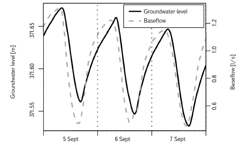
Fig. 1. Typical diurnal fluctuation of groundwater level and baseflow measured in the experimental catchment at the foot of the Alps (modified after [4])
White [1] developed a method to estimate the magnitude of ET on a daily scale based on diurnal fluctuations. The principle of the method is illustrated in Fig. 2. The vertical axis shows the GWL, and the horizontal axis represents time. For a given day, Grec presents a linear extrapolation of expected GWL development in the absence of ET-induced decline. The extrapolation is based on water level development during the night between midnight and 4 a.m., as ET can be considered negligible during this part of the day. ∆S represents the change in groundwater storage during the day (i.e., the change in water level between midnight of the current and previous day). Subsequently, ET is calculated as the sum of Grec and ∆S, multiplied by the specific yield value.
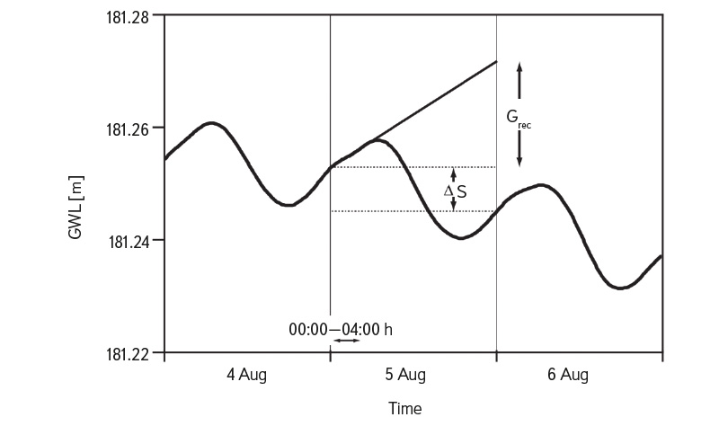
Fig. 2. ET calculation using the White method [1] (modified after [5])
The limitations and behaviour of White’s method were studied in detail, for example, using numerical simulations in Loheide’s 2005 article [6]. The most significant source of error was identified as uncertainty in determining specific yield. A specific yield of 2 % means that if the water level in rock environment drops by 1 m, the amount of water removed from the rock environment is equivalent to removing a 2cm water column from a water volume (e.g., a water tank).
Some authors have proposed alternative methods for estimating ET from GWL fluctuations. In 2008, Gribovszki [4] developed a modification of White’s original method to improve the accuracy of the calculation. Another method was offered by Loheide in an article also published in 2008 [7]. Carlson Mazur, in 2014 [5], subsequently created a modification allowing its application across a wider range of natural conditions. Various methods for calculating ET from GWL fluctuations are discussed in the article by Fahle and Dietrich from 2014 [8]. The values were compared against reference measurements using a lysimeter; the highest correlation with the reference value was obtained using Gribovszki’s method [4].
A significant advance was also made by Malama in 2010 [9]. He derived an analytical solution describing how ET (specified as an input “control function”) manifests in GWL fluctuations (Fig. 3). Malama’s solution [9] also explains the several-hour delay of GWL maxima and minima relative to the solar cycle, which had previously been observed in the field, for example, by Gribovszki [4]. The derived analytical solution can be applied in two ways: to model ET from measured diurnal GWL fluctuations given knowledge of the hydraulic parameters, or, inversely, to infer hydraulic parameters of the environment from diurnal GWL fluctuations given knowledge of ET. In Malama’s article, the developed model was applied to measured diurnal GWL fluctuations, yielding information on ET, hydraulic conductivity, and river stage changes (Fig. 3). This demonstrated that, in principle, both ET and hydraulic parameters can be derived simultaneously from diurnal GWL fluctuations.
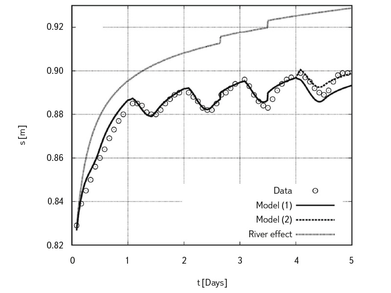
Fig. 3. Model fit of the measured values of diurnal groundwater fluctuation in the vicinity of the river. Model (1) uses the same ET amplitude for the 4th and 5th day, whereas model (2) takes into account the different ET amplitude for the 4th and 5th day. The dotted line represents the effect of fluctuating river stage
Relationship between ET and streamflow
The following group of articles focuses directly on the relationship between ET and streamflow fluctuations. Sometimes this relationship was assessed on a regional scale; an example is 1976 Daniel’s article [10]. This paper addressed the relationship between ET from the aquifer and streamflow in a nearby watercourse, and described an analytical solution that can be used in rainfall-runoff models and GWL models. Another example is Wittenberg’s 1999 article [11]. It determined hydraulic parameters from curves describing the long-term annual decline in streamflow, while observing how recession curves are influenced by ET.
Other articles approached the relationship between ET and streamflow at the catchment scale. An example is Zecharias [12] in 1988 which used a conceptual model to describe the relationship between runoff and aquifer. A significant advance was later made by Fonley [13], who in 2019 derived an analytical relationship for back-calculating ET from records of diurnal streamflow fluctuations (Fig. 4).
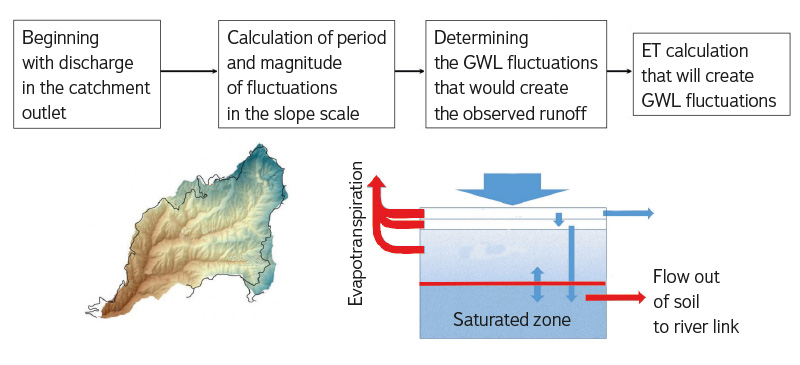
Fig 4. Schematic overview of the Fonley method of calculating ET from diurnal fluctuation of river flow (modified after [13])
ET and fluctuations of GWL combined with streamflow fluctuations
Another group of articles addresses GWL fluctuations caused by ET, while also including observations of the stream flowing through the wetland. Partially, the previously mentioned article by Gribovszki [4] could be included here, whose main contribution was improving methods for calculating ET from GWL fluctuations, but also addressing the relationship with stream level fluctuations. Another example is Yeh [14], whose 2008 article examined the regional-scale soil water balance using 19 years of monthly runoff observations, GWL, and soil moisture. In addition, changes were monitored in the thickness of the subsurface layer influenced by ET.
The relationship between soil moisture and streamflow fluctuations was examined in detail by Moore’s 2011 study [15], conducted in the HJ Andrews experimental forest in western Oregon. He reached the interesting conclusion that, across all time scales, soil moisture correlates very well with the amount of water currently flowing in the stream. The correlation was strongest at high soil moisture levels.
ET, GWL fluctuations, and streamflow combined with independent measurements of vegetation transpiration
The most comprehensive studies of wetland ET are found in articles that monitor not only streamflow and possibly GWL fluctuations but also independently measure vegetation transpiration, for example through sap flow measurements in trees. These articles can be divided into two groups based on location. One group originates from the semi-arid climate of Arizona, the other from the Mediterranean climate of Oregon.
The first group consists of articles from Arizona. They form part of the extensive international SALSA (Semi-Arid Land–Surface–Atmosphere) programme, which focused on human-induced environmental changes in semi-arid regions [16]. ET from waterlogged areas along watercourses (riparian zones) represents an important component of the water balance and was therefore intensively studied within the project using various methods [17]. For example, transpiration of willows and poplars was measured using the sap flow method, and the results were compared with ET values indirectly derived from the water balance [18]. Canopy transpiration derived from sap flow measurements corresponded to values obtained using Raman lidar and was used to calibrate coefficients in the Penman–Monteith method for calculating ET. ET of grasses was also determined using the Bowen ratio method. A summary of these results, together with an estimate of the uncertainty in determining water balance components and a comparison with values obtained using a model, is discussed in detail in the paper by Goodrich (2000) [17].
The second group comprises studies from Oregon (HJ Andrews experimental forest). Important insights are provided in the paper by Bond (2002) [19], where streamflow was measured and correlated with sap flow data from the surrounding vegetation. The measurements were used to estimate the volume of water consumed by ET and to determine the width of the riparian zone from which ET occurred. The study also described in detail the times of year when diurnal fluctuations in streamflow caused by ET were observed.
An interesting contribution from Oregon is the 2007 paper by Wondzell [20], which examined in detail the delay between the daily ET cycle and streamflow fluctuations. It was found that the delay depends on streamflow velocity, more precisely on the speed at which the hydraulic pulse propagates through the channel. When streamflow was fast, the influence of vegetation from different parts of the wetland combined constructively, amplifying the original diurnal signal. In contrast, when streamflow was slow, the influence of vegetation from different parts of the wetland combined destructively (i.e. cancelled each other out), and the original diurnal signal was dampened. Wondzell [20] also mentions diurnal fluctuations in chemical indicators and suggests that they could be subject to a similar delay depending on streamflow velocity.
Another contribution from Oregon is the article by Barnard from 2010 [21]. The aim was to describe the relationship between transpiration and subsurface runoff. To this end, subsurface runoff from the soil, soil moisture, and tree transpiration were measured on a selected small plot. Artificial irrigation was also carried out, and the resulting development of changes was monitored. It was found that the delay of diurnal fluctuation relative to ET depends on soil moisture. In this case, however, Barnard [21] considers it unlikely that the signal from different parts of the catchment could synchronise in such a way that diurnal fluctuations would be observable.
An interesting article from Oregon is also that of Graham from 2013 [22], discussing the frequency of diurnal fluctuations caused by ET. Fifteen different catchments were monitored, and the results were compared with sap flow measurements. Diurnal fluctuations in streamflow caused by ET were observed in all years and across all fifteen catchments, suggesting that this is not merely a special phenomenon limited to a small number of sites.
Review summary
ET in wetland environments remains a highly researched topic today, leading to significant advances in understanding over the past 20 years. GWL diurnal fluctuations caused by ET have been shown to occur across many catchments, as demonstrated by Graham in 2013 [22]. Modifications of the original classic White method have been developed for calculating ET from GWL fluctuations, such as Gribovszki’s method from 2008 [4]. Since the original observations and descriptions, research has progressed to modelling and deriving analytical relationships. An example in the relationship between ET and GWL fluctuations is the article by Malama from 2010 [9], and for the relationship between ET and streamflow fluctuations, the article published by Fonley in 2019 [13]. In the literature, there are also comprehensive studies combining observations of diurnal fluctuations with independent ET determinations by other methods, for example through sap flow measurements in trees. The main groups of articles adopting such a comprehensive approach come from the semi-arid climate of Arizona and the Mediterranean climate of Oregon.
Generally, the current state can be summarised in the following three points. Firstly, since the original observations of changes in water level or flow in wetlands, there has been a tremendous advance in knowledge. Secondly, despite this great progress, it remains necessary to conduct measurements in various locations. These measurements, employing ever-evolving technology, will help verify or supplement hydrological models [13]. The third and very important point is the need to transfer these already acquired insights into the general awareness of experts engaged in practical activities related to hydrology and ecology, who can then apply the new knowledge in everyday practice. This is an important step building on the previous research, which is essential to ensure that current findings are considered in everyday practice. An example of such an effort is this article on wetland ET, which combines a literature review with measurements of GWL fluctuations in a long-term studied wetland in the upper Liběchovka catchment.
Measurement of ET influence in the wetland on the Liběchovka
Following the literature review, a practical demonstration of the influence of ET on a wetland in the western Czech Cretaceous Basin was carried out. GWL fluctuations and runoff from a small wetland were monitored on a minor tributary in the upper catchment of the Liběchovka. It was demonstrated that even under these conditions, diurnal GWL fluctuations caused by ET can be observed. The measurements also provide information on what can be easily used for such monitoring, which conditions must be met, and how this diurnal fluctuation appears in practice.
LOCATION
The measurements were conducted in a wetland in the upper part of the Liběchovka catchment (Fig. 5). It is part of hydrological region 4522 Cretaceous of the Liběchovka and Pšovka. Average annual temperature (calculated based on the period 1981–2010) reaches 8.2 °C, and average annual precipitation totals 595 mm [23].
The site was chosen so that local conditions would not hinder the manifestation of ET. A small watercourse (Soví stream) flows through the wetland, whose main source of water bearing is groundwater from quaternary sandstones; rapid runoff is negligible. Therefore, the watercourse has a stable flow, allowing the impact of water consumption by ET to be clearly observed. The area of the wetland was determined through field survey to be 19,000 m2 [24].
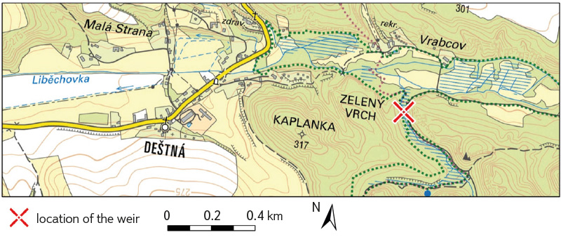
Fig. 5. Wetland area ([24])
METODOLOGY
As a practical demonstration of the influence of ET in the wetland, GWL and soil moisture were monitored. GWL was measured using piezometers, and soil moisture was determined by collecting soil samples.
GWL measurements
This current phase followed up on earlier measurements by the same authors [25] from the second half of summer 2022, which demonstrated that diurnal GWL fluctuations in the monitored wetland are caused by ET and occur on warm, rain-free days. The new study covered the entire summer period, with piezometers installed in different parts of the wetland, enabling observation of the gradual development of diurnal GWL fluctuations from the spring and summer of 2024.
Measurements from the beginning of 2024 until 9 September 2024 were used for the analysis. The location of the newly installed piezometers, which capture GWL spatial variability in the wetland, is shown in Fig. 6. The piezometer referred to as LI2 monitors the conditions in the middle of the lower part of the wetland, close to the constructed weir. The central area of the wetland is represented by the piezometer called Střední mokřad (“Central Wetland”). The piezometer called Boční mokřad (“Lateral Wetland”) describes the edge of the wetland, where the terrain is 2 metres above the valley floor. However, based on the vegetation characteristics, this area is still considered a wetland with GWL close to the surface, which indicates that groundwater flows into the wetland from this side. This is also consistent with the clay layer found at a depth of about 60 cm below the surface, which may form a low-permeability layer along which water flows. Another inflow area to the wetland is represented by the piezometer designated U Studánky (“The Spring”). It was installed at the upper edge of the wetland, near the spring of one of the branches of the watercourse flowing through the wetland.
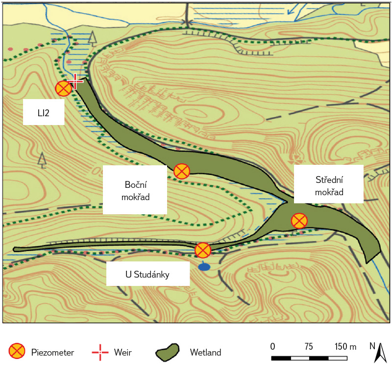
Fig. 6. Location of piezometers in the wetland; for a general overview, location of the weir constructed by the same author during previous work ([25]) is also shown (background map: Base map 1 : 10,000 from [26])
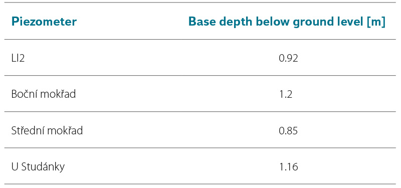
The construction of the piezometers is described in detail in [24].They consisted of pipes with a perforated lower section, in which the GWL was measured using Solinst Logger pressure sensors. To convert the measured pressure to water column height, it was first necessary to subtract the atmospheric pressure from the measured values. Atmospheric pressure was monitored using a Solinst Logger pressure sensor located in the same area as the wetland. For measurement verification, the GWL was also manually measured with a water level meter at the beginning and end of the measuring period. The working names of the piezometers and the depth of their bases below the surface are shown in Tab. 1.
Tab. 1. Depth of the piezometer
Soil moisture measurement
Soil moisture was measured around all installed piezometers, thus covering different parts of the wetland. To avoid disturbance of the soil immediately surrounding the piezometer tube, sampling points were selected approximately 1.5 m from each piezometer. The first sampling took place
in autumn 2023 (12–13 November 2023). This was a cool and wet period, during which it was expected that the soil profile would retain an above-average amount of water and the GWL would be high. The second sampling was conducted during hot summer days in a rain-free period (11th and 12th August 2024),
when it was expected that the soil profile would contain a below-average amount of water and the GWL would be low.
First, a profile was excavated to a depth where water began to visibly seep from the walls, and the characteristics of the individual layers were roughly described. Subsequently, samples were taken. The sampling depths were adjusted to ensure that prominent soil layers were captured. During the second sampling, it was necessary to select a location near the piezometer that had not been disturbed during the previous sampling; therefore, the profiles for the same piezometer slightly differ between the first and second samplings. Kopecký cylinders with a volume of 100 cm³ were used for sampling, driven in horizontally. Within each profile, one sample was taken from each observed layer to determine specific yield. Immediately after sampling, the cylinders were sealed with lids, wrapped in foil, and placed in plastic bags to prevent moisture loss. As soon as the samples returned from the field, they were weighed on scales with an accuracy of 0.1 g. Subsequent weighing was conducted on the same scales.
The first step in sample processing was to determine saturated moisture content. Cylinders containing the samples were placed individually in a container, filled with water from the bottom, and left submerged for three days. They were then removed from the container and weighed. In two exceptional cases, a non-negligible loss of material occurred from the sample, which distorted the moisture content in the saturated state (a note has been added in the resulting graphs for the respective samples). The second step was to measure the weight of the dried soil. First, the sample was dried for several days at room temperature, then for 1.5 weeks in an oven at 105 °C, and finally it was weighed immediately after removal from the oven to prevent it from absorbing atmospheric moisture.
From the measured data, the volumetric moisture content of the sample at the time of collection (θodb) and the saturated (volumetric) moisture content of the sample (θsat) were calculated as follows:
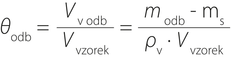 (1)
(1)
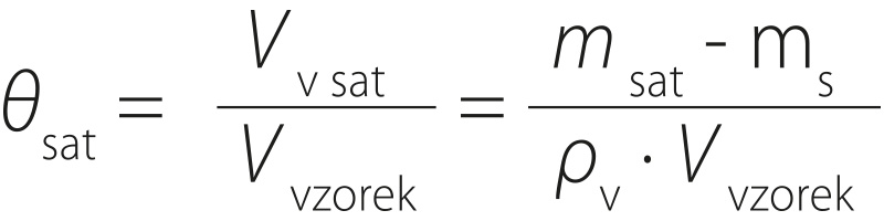 , (2)
, (2)
where:
V v odb is the volume of water in the sample at the time of collection
V v sat the volume of water in the sample in the saturated state
V vzorek the volume of the collected sample (100 cm³)
m odb the weight of the sample at the time of collection
m s the weight of the dried sample
m sat the weight of the sample in the saturated state
ρ v the density of water (1,000 kg · m-3)
Subsequently, the resulting moisture values were converted from decimal numbers to percentages.
Estimation of ET from GWL fluctuations
In the first step, the specific yield of the soil layers in which diurnal GWL fluctuations occur was estimated based on soil moisture measurements. This allowed the measured GWL fluctuations to be converted into the amount of water gained or lost from the groundwater during level changes in subsequent data processing steps. For the estimation of specific yield, only those piezometers were selected where, during soil profile sampling, few heterogeneous layers were detected at depths around the GWL.
The calculation of ET from diurnal GWL fluctuations was performed in a simplified manner based on the original classical method by White [1]. The principle of the method is summarised in Fig. 2 in the review section of this article. First, the average hourly change in GWL (r) was calculated based on the interval between midnight and 4 a.m. This value reflects the long-term GWL trend without the influence of daytime ET. Subsequently, the daily change in soil water storage (∆Z) was calculated as:
 , (3)
, (3)
where:
h1 is the GWL at midnight of the current day
h2 the GWL at midnight of the following day
A positive value of ∆Z indicates a drop in GWL during the day, meaning a loss of water from the environment.
In the next step, ET was calculated and expressed as the height of the water column per day:
![]() , (4)
, (4)
where:
S is the specific yield
r average change in GWL without the ET influence
∆Z zchange in storage over a day
The obtained ET value was converted from the water column form to a flow rate form (volume of water consumed per unit of time). The resulting wetland ET value was calculated as the arithmetic mean of the individual values from each piezometer. This value was then compared with ET estimates based on streamflow fluctuations and the Oudin method for calculating PET, which had been conducted by the same authors on earlier data from the same site [25].
The average ET value calculated from the piezometers using White’s method was designated as ETprům. However, some piezometers were excluded from the ET calculation due to the presence of many different soil layers. Retrospective estimates were made for these piezometers to determine the specific yield required for the ET value calculated by the White method from GWL fluctuation to equal ETprům. This calculation was performed using the Solver function in MS Excel.
RESULTS
GWL measurement
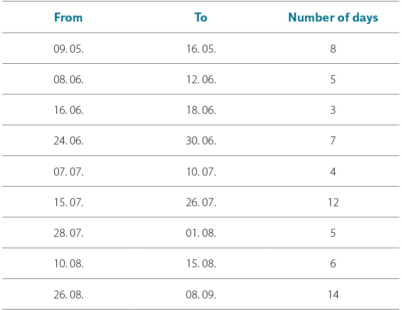
From the measured data, periods were selected during which significant diurnal GWL fluctuations occurred over several days (Tab. 2). There were eight such periods, with the duration of individual episodes ranging from three to fourteen days, and fluctuations were evident at all measured locations within the wetland. During these periods, the water level of the small watercourse at the weir also fluctuated. However, the amplitude of stream level fluctuations was significantly smaller – up to a maximum of 2.5 cm in peak summer – compared to GWL fluctuations, which reached up to 14.5 cm in peak summer at Střední mokřad piezometer.
Tab. 2. Periods with diurnal fluctuation in groundwater level in the wetland (2024)
The first significant signs of diurnal GWL fluctuations were observed at the beginning of May (A in Fig. 7). During the eight-day period from 9 to 16 May, fluctuations were greater in the central part of the wetland (Střední mokřad piezometer) compared to fluctuations at other locations within the wetland. Another period with clearly visible GWL fluctuations was the first half of June, specifically from 8 to 12 June (B in Fig. 7) and from 16 to 18 June. The amplitude of fluctuations was more pronounced compared to May, especially in the case of Střední mokřad piezometer. An exception was U Studánky piezometer, where fluctuations were smaller compared to the other piezometers.
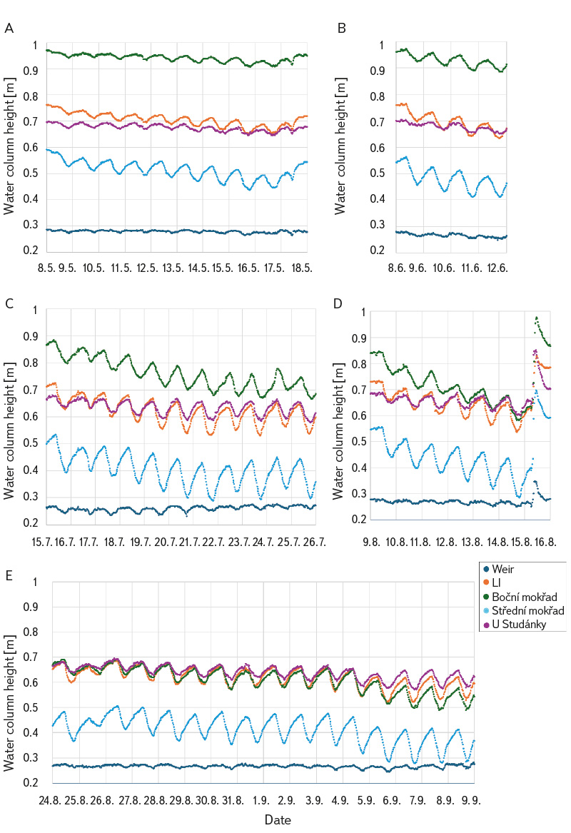
Fig. 7. Diurnal fluctuation in groundwater level in early spring (A), late spring (B), midsummer (C, D), and the end of summer (E)
From the end of July, marked diurnal fluctuations in water level were observed in all piezometers (C and D in Fig. 7). These occurred during the periods from 24 to 30 June, 7 to 10 July, 15 to 26 July, 28 July to 1 August, and 10 to 15 August. However, in the case of the U Studánky piezometer, the amplitude of the fluctuations remained lower. The longest continuous period of diurnal GWL fluctuation occurred over 14 days at the end of summer, from 26 August to 8 September (E in Fig. 7).
Soil moisture measurements
The soil moisture measurement results are presented in Tab. 3 and summarised in Fig. 8. The moisture content of sandy layers during sampling was around 40 %, while the moisture content of clayey-silty layers was significantly higher, generally between 70 and 80 %.
Soil profiles sampled in autumn and summer at the same piezometer were only a few metres apart, yet the layer composition often differed significantly. This indicates pronounced variation between soil profiles at different places within the wetland, which is a consequence of the watercourse dynamic activity. Simultaneously, this generally implies that it is difficult to determine representative hydraulic parameters for such environments, for example for the purposes of accurate modelling.
During autumn sampling, GWL was higher than in summer. In both periods, however, soil throughout the entire profile was very close to saturation. The difference between moisture content at the time of sampling and saturated moisture content was greatest in the surface layers, but even in this case it did not exceed 4 %.
The measurement error in determining soil moisture was estimated to range between 1 and 2 %. This is based on the fact that, in some samples, the measured moisture content at the time of sampling exceeded the saturated moisture content, or that layers below the GWL were not saturated. A difference value of 0 between saturated and sampled moisture content indicates that the sample’s moisture content at the time of sampling was equal to or greater than the saturated moisture content.
In one case, it was found that a sample taken well below the GWL was 5 % below saturation; in another, the moisture content of the sample significantly exceeded the saturated moisture content (by 5 %). These values were considered to be processing errors caused by partial water loss from the sandy sample during handling prior to weighing. In the case of a third sample, it was found that just below the GWL the sample was 3 % below saturation. This was considered to be the result of GWL recorded from the nearby piezometer not exactly matching the GWL at the location of the sampled profile, and the respective sample was in fact taken from above the water level.
Tab. 3. Results of soil moisture measurements
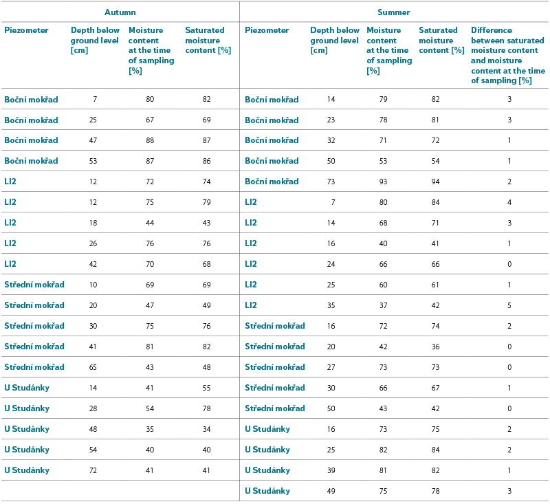
Fig 8. Measuring soil moisture content in the wetland (in the profile description, soil horizons are described in brackets according to the soil classification)
Estimation of ET from GWL fluctuations
The first step was to determine specific yield of the soil layers at the GWL depth. Summer moisture measurements were used, as diurnal GWL fluctuations were recorded during the warm part of the year. From the sampled profiles, the Boční mokřad and U Studánky piezometers were selected for analysis, as the soil composition at these sites showed little variation with depth. Samples were taken from layers above the GWL, and specific yield was determined as the difference between the saturated moisture content and the moisture content at the time of sampling. Using this method, specific yield was estimated at 2 %, with an absolute error of ±1 %.
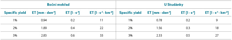
In the second step, White’s method [1] was applied to calculate ET based on the measured diurnal fluctuations in GWL at the U Studánky and Boční mokřad piezometers. The results are summarised in Tab. 4. The values presented are average ET calculated based on eight periods during which significant GWL fluctuations occurred over several days. The final ET estimate was calculated as the arithmetic mean of the values obtained from both piezometers and reached 20 l ∙ s-1 ∙ km-2, with a range of ± 10 l ∙ s-1 ∙ km-2 considering a specific yield variation of ± 1 %.
In the final step, the obtained ET value was compared with the results of ET estimation by a different method, carried out by the same authors in the same wetland [25]. In the referenced study, ET was calculated based on fluctuations in streamflow, under the assumption that the highest daily flow represents discharge unaffected by ET. Using this method, ET was determined to be 11 l ∙ s-1 ∙ km-2. Based on the calculation of PET using Oudin’s method, the study reported an average ET value of 25 l · s-1 · km-2. These results from 2022 are consistent with the ET values obtained using White’s method – 20 l ∙ s-1 ∙ km-2 – within the accuracy limits of the specific yield estimate.
In order for the ET value of 20 l ∙ s-1 ∙ km-2, as determined by White’s method, to be valid also for the Střední mokřad piezometer, it was retrospectively calculated that the specific yield for this piezometer would need to be approximately 2 %. In the case of the LI2 piezometer, the same retrospective approach indicated a specific yield of around 1 %. Both values fall within the expected range of specific yield. In future measurements, it will be beneficial to compare the determined specific yield value with specific yield obtained experimentally by other means – for example, through a pumping test with a small volume of water extracted from piezometers, while monitoring the drawdown and geometry of the cone of depression using additional temporarily installed piezometers in the vicinity. This approach should lead to a significantly more accurate determination of specific yield.
Tab. 4. ET in the wetland calculated using the White method
DISCUSSION
The measurements presented build upon previous research steps carried out by the same author at the same site. The results are consistent with findings from international studies presented in the first (review) section. In Pátek’s 2022 study [24], diurnal GWL fluctuations and streamflow were detected at a single location within the wetland. Daily amplitude of fluctuations (difference between maximum and minimum GWL on a given day) increased with higher temperatures. This relationship was more apparent when only rain-free days were considered, and it was most pronounced on days with more than nine hours of sunshine. These findings confirmed the assumption that the detected fluctuations were caused by ET influence. In the subsequent article by Pátek and Bruthans from 2023 [25], diurnal streamflow fluctuation was used to estimate the amount of water consumed by vegetation, and the result was compared with the theoretical method of calculating PET using Oudin’s approach. A delay was also observed between the timing of streamflow minimum and maximum and the solar cycle. The typical timing of the daily streamflow maximum (around 08:00) and minimum (around 16:30) is consistent, for example, with the findings of Gribovszki [3], obtained from an experimental catchment in the foot of the Alps, where in August the maximum flow occurred around 07:00 and the minimum around 16:00.
In the monitored wetland, the previous research steps were expanded by simultaneously observing the GWL across the entire area, which enabled an assessment of the spatial variability of diurnal GWL fluctuations. The fluctuations occurred uniformly and synchronously throughout the wetland, including its peripheral parts, with the most pronounced effect observed in the central area.
Soil moisture measurements yielded further interesting findings. The soil above the GWL was close to saturation, even during the summer months when ET was intense. It is surprising that, despite the presence of an unconfined aquifer, specific yield is very low – only a few per cent. This is due to the predominance of fine-grained material, in which the vast majority of pores are filled with water (capillary fringe), and only a very small volume contains air.
The high moisture present throughout the entire soil profile allows ET to have a more pronounced effect on GWL fluctuations. The primary reason for this is the easy availability of water to plant roots. The second reason is that only a small amount of water is needed to fully saturate the soil above the GWL, causing the GWL to rise (specific yield is therefore low, ranging from 1 to 4 %). As a result, a small volume of added or removed water produces pronounced vertical movements of the GWL. High soil moisture in summer also means that water is readily available even during dry periods, when ET from areas outside the wetland is limited by water scarcity. Consequently, the relative impact of secondary ET from the wetland on the landscape’s water balance is greater.
The measured data allowed only an approximate estimate of specific yield. Differences between the moisture content of saturated samples and that of samples at the time of collection were in the single digit per cent range, roughly comparable to the accuracy of the method used. In addition, the properties of the individual soil profile layers varied significantly. This strong spatial variability in specific yield values suggests that even taking multiple Kopecký cylinders from a single specific depth within a given profile would not lead to a significant improvement in accuracy. This indicates that, in future studies, it will be more appropriate to use other methods for determining specific yield in the wetland, such as a miniature pumping test (pumping in ml · s-1 and water level drawdown in decimetres around the piezometer). An additional advantage of this method is that it reflects the overall behaviour of a larger volume of the environment and is therefore less sensitive to the heterogeneous soil profile composition in the wetland, which is influenced by the watercourse dynamic activity.
Diurnal fluctuations caused by ET were observed in the wetland both in streamflow (i.e., a decrease in flow during the day compared to night) and in GWL fluctuations (a drop in GWL during the day compared to night). The connection between the fluctuations of these two variables stems from the fact that the main source of water for the small stream flowing through the wetland is groundwater. Measuring fluctuations in GWL was easier compared to measuring fluctuations in streamflow because the vertical range of GWL movement was greater than that of the stream’s surface level fluctuations, making the measurements relatively more precise. In environments where the GWL is close to the surface and the time lag between GWL fluctuations and streamflow is small, this finding suggests an alternative, simple method to measure streamflow with minimal instrumentation requirements. The close relationship between GWL and streamflow is also consistent with the results of Moore [15]; here, a strong correlation was described between current streamflow and soil moisture, with the relationship found to be more accurate at higher soil moisture levels.
The conducted measurements also demonstrate how diurnal GWL fluctuations can be detected using relatively simple and low-cost equipment. The measurements required only piezometers consisting of pressure sensors inserted into perforated pipes buried in the ground, whose installation involved only minimal environmental disturbance. The low maintenance requirements enable long-term monitoring, which could be used, for example, to assess the wetland condition, including the early detection of changes such as drought or tree dieback. Adding a simple weir to the measurement network allowed manual volumetric streamflow measurement. A flow rating curve was established, and the water level records captured by the sensors could be converted into streamflow records [25].
CONCLUSION
The literature review section of the article contains an overview of research focused on the impact of ET in wetlands on the water balance. The research can be divided into four groups, describing a spectrum of articles ranging from those examining detailed fluctuations of groundwater level (GWL) to more comprehensive studies combining GWL fluctuations with streamflow and, in some cases, also with measurements of vegetation transpiration by other methods, such as measuring sap flow in trees.
Theoretical knowledge was complemented in the second part by practical measurements illustrating the situation in the western part of the Czech Cretaceous Basin. The ET influence on the wetland in the upper catchment of the Liběchovka was monitored. Consistently with the results of the review conducted in the first part of the work, three main observations were made:
- a significant influence of secondary ET in the wetland on water balance,
- diurnal GWL fluctuations which, due to ET, occur simultaneously throughout the wetland during the summer months,
- a temporal delay of the diurnal GWL fluctuations and streamflow relative to the solar cycle.
Based on diurnal fluctuations, the wetland ET was determined to be 20 l ∙ s-1 ∙ km-2. This is an average value representing the warm periods of the summer, during which significant diurnal GWL fluctuations were observed over several days. This is consistent with the results of previous measurements at the same site by the same authors [25], where ET was derived from fluctuations in the flow of the small watercourse passing through the wetland and from Oudin’s method for calculating PET.
The necessity of considering the influence of wetland ET on the water balance in Central Europe was thus supported, as demonstrated by Bruthans in his 2020 study [2], based on streamflow measurements. From this study and other similar studies, the following important general conclusion emerges, carrying significant implications for hydrological practice. Wetlands and similar environments are not elements that retain water in the landscape; rather, they are environments where water is intensively consumed by vegetation and, under high summer temperatures, rapidly lost to the atmosphere.
Acknowledgements
Field measurements were supported by the Technology Agency of the Czech Republic project No. SS02030040 „Prediction, evaluation and research of the sensitivity of selected systems, the impact of drought and climate change in the Czech Republic“.
The Czech version of this article was peer-reviewed, the English version was translated from the Czech original by Environmental Translation Ltd.
