ABSTRACT
The study quantifies changes in the 100-year design quantile of short-duration precipitation at ungauged locations in the Czech Republic and analyses the uncertainty structure of these estimates under climate change conditions. Reference IDF curves were derived using regional frequency analysis based on the index-flood concept, employing the GEV distribution with parameter estimation using the method of L-moments. Future changes were determined from a multi-model ensemble of CORDEX regional climate projections for the RCP2.6, RCP4.5, and RCP8.5 scenarios for the periods 2035–2065 and 2070–2100.
Under the RCP8.5 scenario (2070–2100), the mean relative change in
the 100-year hourly quantile is approximately 52 %, with the 5th–95th percentile range spanning from −7 % to +126 %. In the period 2035–2065, differences among emission scenarios are smaller than the internal variability of the models, whereas in the second half of the century the emission trajectory becomes the dominant source of projection divergence. Relative amplification is greater for shorter durations, indicating a disproportionate sensitivity of short-term extremes.
The analysis shows that uncertainty at high return periods is strongly influenced by the estimation of the GEV shape parameter, where small differences lead to nonlinear growth in extrapolated quantiles. The detected intensification of extreme precipitation is consistent with the expected thermodynamic amplification of the hydrological cycle; however, the ensemble spread highlights substantial structural uncertainty in regional climate models.
The results indicate that the use of historical IDF curves without accounting for climate change may lead to a systematic underestimation of design values, particularly for infrastructure with a long service life.
INTRODUCTION
Extreme precipitation events are of the most significant hydrometeorological phenomena affecting public safety, the functioning of technical infrastructure, and the economic stability of regions [1]. Under Central European conditions, flash floods and local inundation have long been associated primarily with short-duration intense rainfall events, the impacts of which are intensified by urbanisation and changes in land use. The increasing proportion of impervious surfaces, river channel modifications, and the concentration of built-up areas accelerate the runoff response of catchments and increase the sensitivity of the landscape to extreme precipitation episodes.
The design of technical measures such as sewer systems, retention reservoirs, dry polders, and blue-green infrastructure elements is therefore based on the statistical description of extreme precipitation [2]. In practice, design quantiles expressed through intensity–duration–frequency (IDF) curves are used as the principal tool for the dimensioning of water management structures [3, 4]. These curves are usually derived from historical precipitation time series and implicitly assume a stationary climate regime [3].
The assumption of stationarity, however, is no longer defensible in the context of ongoing climate change [1]. Increasing concentrations of greenhouse gases lead to atmospheric warming, which is associated with changes in the hydrological cycle [5]. Climate models as well as observed trends indicate an intensification of extreme precipitation in many regions of the world [1, 6]. The physical basis of this intensification is linked to the Clausius–Clapeyron relationship, according to which the maximum water vapour content of the atmosphere increases by approximately 7 % per 1 K of warming [5, 6]. A higher water vapour content creates the potential for more intense precipitation events, particularly those of a convective nature [6].
Although the physical mechanism responsible for the intensification of extreme precipitation is relatively well understood, its quantification at the regional and local levels is subject to considerable uncertainty [1]. This uncertainty arises from several sources, namely structural differences among climate models, uncertainty associated with emission scenarios, and internal climate variability [7]. From the perspective of water management practice, however, not only the mean change in the design quantile is important, but above all its upper bound, which represents the potential risk of infrastructure underdesign.
Another significant problem is the limited availability of long-term high-quality precipitation measurements. In many locations, sufficiently long time series enabling reliable estimation of high return periods are not available. The extrapolation of a 100-year or 200-year quantile from a short time series is statistically unstable and sensitive to individual extreme events [2, 8]. Regional frequency analysis (RFA) represents a methodological approach that mitigates this problem through the sharing of information among climatically similar locations [9]. By separating the regional shape of the distribution from the local scale, it enables a more robust estimation of extreme quantiles even in areas without direct measurements or with limited data availability [9].
The literature contains numerous studies addressing changes in extreme precipitation in the context of climate change; however, fewer studies systematically combine regional frequency analysis with a multi-model ensemble of climate projections and explicitly quantify the uncertainty associated with high return periods [3, 10, 11]. In particular, insufficient attention has been paid to the question of how large the uncertainty of the 100-year design quantile is and how its structure changes depending on the time horizon and emission scenario [7].
The present study aims to partially fill this gap. The methodology described below was applied to three pilot locations (Bukovno, Pečky, and Běchovice). The main research questions can be formulated as follows:
- What is the magnitude of the change in the 100-year design precipitation under future climate conditions?
- What is the spread of the climate projection ensemble, and how does it evolve over time?
- Is the observed intensification of extreme precipitation consistent with the theoretical Clausius–Clapeyron scaling?
Answers to these questions are of direct relevance to the dimensioning of water management infrastructure as well as to the strategic planning of adaptation measures. The study therefore combines regional frequency analysis with a multi-model ensemble of regional climate projections and focuses not only on the estimation of future IDF curves, but especially on the systematic quantification of their uncertainty [7, 10, 11].
DATA
Observed precipitation data
Observed data on short-duration precipitation totals from the network of stations operated by the Czech Hydrometeorological Institute (CHMI) were used for the construction of reference IDF curves for the three pilot locations [12, 13]. Only stations with time series exceeding 30 years in length were included in the analysis, representing the minimum duration required for a more robust estimation of high return periods within the framework of block maxima analysis [2, 8]. The selection of stations was further restricted to locations with sufficient measurement continuity and a minimal proportion of missing data.
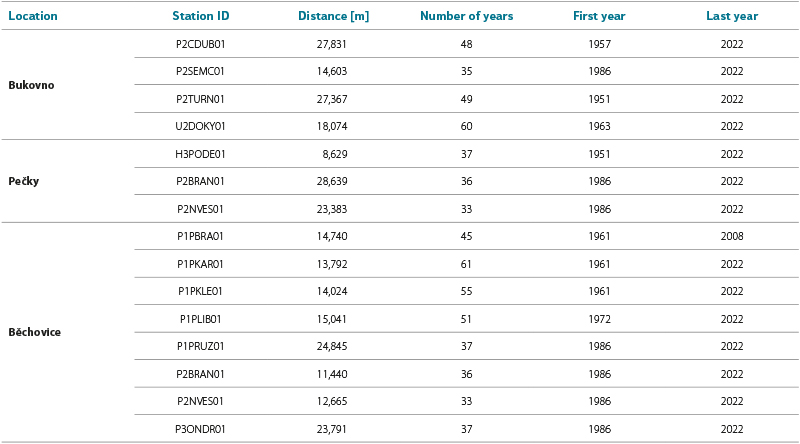
The primary criterion for station selection was their spatial proximity to the analysed locations, defined as a circular buffer with a radius of 30 km. Only stations located within this radius and simultaneously meeting the requirement of a time series of annual maxima of at least 30 years were included in the regional analysis. The minimum record length was selected with regard to the stability of the estimation of the parameters of the GEV (General Extreme Value) distribution and to the limitation of uncertainty associated with the extrapolation of high return periods. This approach assumes that stations meeting both criteria exhibit sufficient climatic similarity and statistical robustness for the application of regional frequency analysis. The stations used are shown and described in Fig. 1 and Tab. 1.
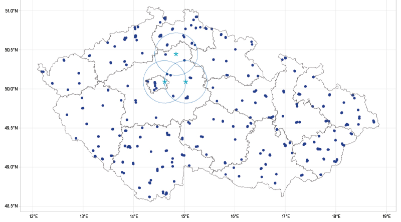
Fig. 1. Selection of stations for RFA – locations marked with a star indicate pilot sites, points marked with a dot represent rain gauge stations CHMI, and circles denote the 30km buffer
Tab. 1. Meteorological stations used for RFA, their distances to the pilot locations, and the length of the annual maxima time series
The block maxima method was used for the application of extreme value theory [2, 8]. For each duration (5 minutes to 24 hours), annual maxima were extracted from the time series. This approach is consistent with the classical formulation of EVT (Extreme Value Theory) and allows the direct application of the GEV distribution [8]. The resulting set of annual maxima constituted the input for the regional frequency analysis and for the estimation of the parameters of the GEV distribution in the reference period [8, 9].
CORDEX climate projections
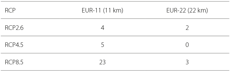
Future changes in design precipitation were derived from regional climate projections of the CORDEX (Coordinated Regional Climate Downscaling Experiment) initiative [14]. Models from the European EUR-11 (horizontal resolution of approximately 11 km) and EUR-22 (resolution of approximately 22 km) domains were used [15]. The higher spatial resolution allows a more detailed representation of orography and regional circulation processes influencing extreme precipitation.
The ensemble included multiple combinations of global climate models (GCMs) and regional climate models (RCMs). This multi-model approach makes it possible to capture structural uncertainty arising from differences in the dynamical cores of the models, the parameterisation of cloud processes and convection, and atmosphere–surface interactions [7, 16]. Each GCM–RCM combination represents one realisation of future climate, while the complete set of realisations constitutes the ensemble. An overview of the ensemble combinations used is presented in Tab. 2.
Tab. 2. Composition of the ensemble of projections used (number of unique GCM–RCM combinations) by RCP scenario and domain
Three time periods were evaluated:
- the reference historical period (model simulation corresponding to past climate conditions),
- the near-future period 2035–2065,
- the distant-future period 2070–2100.
For future projections, the RCP2.6, RCP4.5, and RCP8.5 emission scenarios were analysed, representing different trajectories of greenhouse gas concentration development [17, 18]. The RCP2.6 scenario assumes rapid stabilisation of emissions, RCP4.5 an intermediate stabilisation trajectory, and RCP8.5 a scenario of continuing emission growth [18].
Hourly precipitation data from climate models, expressed in units of kg ∙ m-2 ∙ s-1, were used and converted to precipitation totals before being aggregated to the required durations. For each grid point corresponding to the analysed pilot sites, a time series of annual maxima was extracted from the regional models using a procedure analogous to that applied to the observed data [8].
To reduce the influence of systematic model biases, the future change in the design quantile was expressed in relative form [3]:
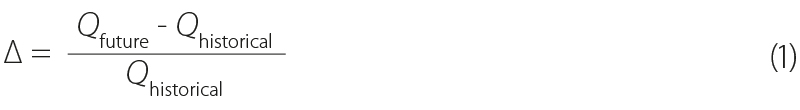
This approach assumes that the systematic model bias is largely consistent between the historical and future periods, thereby allowing the analysis to focus on the relative change in extremes rather than on their absolute values [16]. The relative changes were subsequently applied to the reference IDF curves derived from observed data, yielding future design values for the individual emission scenarios for both projection periods [12, 13]. This procedure made it possible to link the local statistical behaviour of extreme values derived from observed data with future climate projections, while simultaneously systematically quantifying the ensemble spread as a measure of model uncertainty [7].
Theoretical framework
Extreme value theory
Extreme value theory (EVT) represents a statistical approach based on the asymptotic properties of extremes, intended for modelling the behaviour of maxima of random variables [2, 8]. Whereas the classical central limit theorem describes the limiting behaviour of sums, EVT focuses on the limiting properties of extremes. For independent and identically distributed random variables X1,…, Xn, it holds that for suitably normalised maxima Mn = max (X1, …, Xn), the corresponding distribution function converges to the Generalised Extreme Value (GEV) distribution [8].
The distribution function of the GEV distribution is given by the following equation:
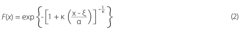
where:
ξ is the location parameter
α > 0 the scale parameter
κ the shape parameter [8]
The shape parameter determines the thickness of the right tail of the distribution. For κ > 0, the distribution has a heavy tail (Fréchet type); for κ = 0, it reduces to the Gumbel type; and for κ < 0, it has a finite upper bound (Weibull type) [8]. Estimation of this parameter is crucial for the extrapolation of high quantiles, because small changes in κ may lead to substantial differences in the estimation of 100-year or 200-year extremes [2, 8].
Quantiles of the GEV distribution can be expressed by inversion of the distribution function:
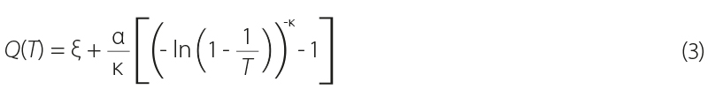
where:
T is the return period [8].
This explicit formulation allows the direct calculation of design values following parameter estimation.
Regional frequency analysis
Regional frequency analysis (RFA) is a methodology developed to increase the robustness of the estimation of extreme quantiles in situations with limited time-series length [9]. The basic idea is the sharing of information among stations exhibiting similar statistical behaviour of extremes [9].
The index-flood concept assumes:
where:
Qi(F) is the quantile at location
µi the local scaling factor
q(F) the dimensionless regional growth curve common to the entire region [9]
The scaling factor µi is typically defined as the first L-moment (analogous to the sample mean) of annual maxima [9, 19]. For the pilot locations without direct measurements, the scaling factor was estimated using the IDW (Inverse Distance Weighting) method. This method allows the interpolation of quantile values from surrounding gauged stations on the basis of a weighted average of the values, where the weight assigned to each station is inversely proportional to the distance from the analysed location. The distances of the individual stations used for the three pilot locations are presented in Tab. 1. By normalising the data from individual stations by their local scale, a dimensionless dataset is obtained, from which the regional shape of the distribution is subsequently estimated [9].
Homogeneity of the region was evaluated within the framework of regional frequency analysis based on L-moments according to [9]. For each duration, the L-moment ratios of individual stations were first calculated, and the expected variability of a homogeneous region of the same size was subsequently estimated using Monte Carlo simulations (1,000 realisations). On this basis, H-statistics (H1, H2, H3) were determined (a summary is provided in Tab. 3) quantifying the deviation of the observed inter-station variability from the variability of the simulated homogeneous region.
According to the interpretation criteria of [9], H < 1 indicates a homogeneous region, 1 ≤ H < 2 weak heterogeneity, and H ≥ 2 a heterogeneous region.
To identify potentially inconsistent stations, the discordancy measure was applied. Its values remained, in most cases, below the critical threshold (1.33 for the three-member subregion and 2.33 for the broader region), indicating no pronounced outliers in the L-moment space. Overall, the region can be considered sufficiently homogeneous for the application of regional frequency analysis, while acknowledging slightly increased variability for longer durations.
Tab. 3. Summary of regional statistics for the Bukovno, Pečky, and Běchovice regions; ranges of heterogeneity metrics are reported
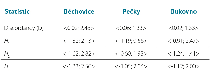
The overall assessment indicates that the Bukovno area is predominantly homogeneous from the perspective of regional frequency analysis, although with locally increased heterogeneity, particularly according to the statistic H1 and marginally also H3. The Pečky area appears to be the most homogeneous of the three locations, with no exceedance of the critical discordancy threshold and only indications of weak to moderate heterogeneity in H2 and H3. In contrast, Běchovice exhibits the highest degree of spatial heterogeneity, reflected both by isolated exceedances of the critical discordancy threshold and by elevated values of the H2 and H3 statistics.
RESULTS
The theoretical framework based on the GEV distribution and regional frequency analysis made it possible to translate climate projections into changes in the design quantiles of extreme precipitation. The following section therefore presents a quantification of these changes, focusing on the magnitude of the 100-year quantile and on the structure of uncertainty arising from the multi-model ensemble.
Change in the 100-year hourly quantile
The relative change in the 100-year hourly quantile Q100 exhibits a systematic dependence on both the emission scenario and the time horizon. In the period 2035–2065, differences among the RCP scenarios are smaller than the internal variability among individual realisations within the same scenario. In the distant period 2070–2100, a pronounced divergence among the scenarios becomes apparent.
Under the RCP8.5 scenario (2070–2100), the mean relative change in Q100 amounts to 52 % with a standard deviation of 41 %. The interval between the 5th and 95th percentiles ranges from −7 % to +126 %. The median change is approximately 47 %. Approximately 80 % of the realisations exhibit a positive change.
For the RCP2.6 scenario (2070–2100), the mean change is approximately 19 %, and the uncertainty interval is substantially narrower. The difference between the mean changes under the RCP8.5 and RCP2.6 scenarios in the second half of the century exceeds 30 percentage points.
Values exceeding 100 % are generated by a limited number of realisations and correspond to cases with a positive shape parameter κ, implying a heavy right tail of the GEV distribution. The distribution of changes across scenarios and periods is shown in Fig. 2, which illustrates the pronounced widening of the ensemble spread under the RCP8.5 scenario (2070–2100).
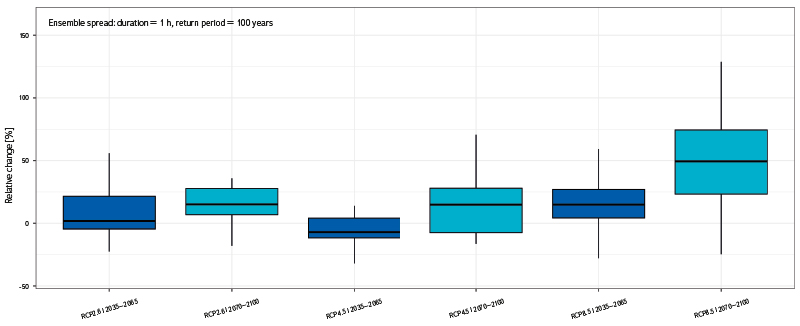
Fig. 2. Relative change in the 100-year hourly quantile (Q₁₀₀, 1 h) across RCP scenarios and time horizons for three pilot areas. Box plots represent individual GCM–RCM realizations (37 in total) within the 5th–95th percentile range; the box indicates the interquartile range and the black line denotes the median. Time horizons are distinguished by colour – dark blue (2035–2065) and light blue (2070–2100). The ensemble spread is substantially wider under the RCP8.5 scenario (2070–2100), where the upper bound exceeds 100 %
Dependence on duration
The relative change in extreme precipitation exhibits a decreasing trend with increasing duration. Under the RCP8.5 scenario, representing a high-emission scenario used primarily to illustrate the upper bound of climate impacts (2070–2100), the mean change is approximately:
- 1 h: 52 %,
- 6 h: 39 %,
- 24 h: 28 %,
- 48 h: 28 %.
This gradient is also evident from the IDF curves for the same scenario variant shown in Fig. 3, where the intensification is more pronounced for shorter durations.
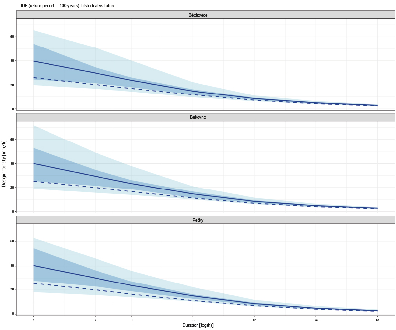
Fig. 3. Comparison of historical and future IDF curves (T = 100 years) for the pilot locations Bukovno, Pečky, and Běchovice. The solid line represents the median of the RCP8.5 (2070–2100) projections, while the dashed line corresponds to the reference period. The lighter blue area indicates the 5th–95th percentile range of the ensemble, and the darker blue area shows the 25th–75th percentile range
The range between the 5th and 95th percentiles is wider for shorter durations. Relative uncertainty therefore increases with the intensity of the extreme event.
Influence of the shape parameter κ
The sensitivity of high quantiles to the shape parameter increases with the return period T. It follows from the GEV quantile function (3) that ∂ Q / ∂ κ increases with T. Small differences in the estimation of κ therefore lead to substantial differences at high return periods.
Realisations with κ > 0 generate more rapid growth of Q(T) and explain the upper part of the ensemble spread. This effect represents a structural source of extrapolation uncertainty. The increase in relative uncertainty with return period is documented in Fig. 4, where the spread of projections systematically increases with increasing return period.
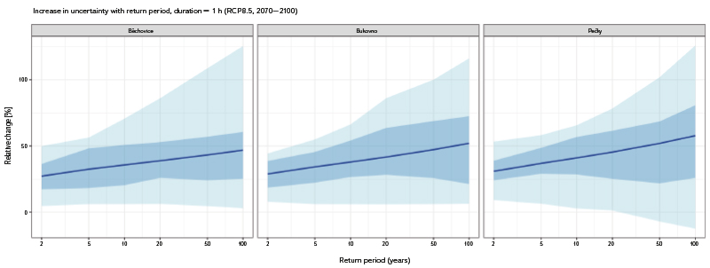
Fig. 4. Dependence of the relative change in the design quantile on return period (logarithmic scale) for a 1-hour duration under the RCP8.5 scenario (2070–2100). Solid lines represent the mean change, the light blue area indicates the 5th–95th percentile range of the ensemble, and the darker blue area shows the 25th–75th percentile range. The spread among realizations increases with return period, reflecting the sensitivity of the extrapolation to the shape parameter κ
DISCUSSION
Dominant sources of uncertainty
The nature of uncertainty differs depending on the time horizon. In the near-future period, structural model variability is dominant, whereas in the distant-future period the divergence among emission scenarios becomes increasingly important. This result is consistent with the general conclusions of climate projection studies.
It should be emphasised that the presented spread includes only the variability among model realisations. Uncertainty associated with the estimation of the GEV parameters (e.g. confidence intervals of κ) is not explicitly quantified here and may further increase the overall uncertainty.
Interpretation of high relative changes
Relative changes exceeding 100 % represent the upper part of the projection distribution and are not representative of the centre of the ensemble. Their occurrence is associated with a combination of a strong climate signal and positive κ.
From a purely thermodynamic perspective, Clausius–Clapeyron scaling would imply an intensification of approximately 28 % for a warming of about 4 K [5, 6]. The mean value of 52 % under the RCP8.5 scenario (2070–2100) exceeds this simple scaling, suggesting that, in addition to thermodynamic intensification, dynamic changes in circulation, changes in convective organisation, or nonlinear responses of extremes may also play a role.
Since the study does not perform an explicit analysis of the underlying dynamical mechanisms, this interpretation should be regarded as a hypothesis consistent with the literature rather than as direct evidence.
Implications for infrastructure design
The use of historical IDF curves without accounting for climate change leads, under higher-emission scenarios, to a systematic underestimation of extreme precipitation volumes.
At the same time, the ensemble mean cannot be regarded as a sufficient representation of risk. Design values should reflect the full range of projections and should be assessed in the context of the acceptable level of risk and the service life of the infrastructure.
Application framework of the study
The methodology and the selection of pilot locations are directly linked to the objectives of the project Adaptation of Urbanised Areas to Flash Floods and Drought (SrUrb, No. SS06010386), funded by the Technology Agency of the Czech Republic under the Environment for Life programme. The aim of the project is to support decision-making processes related to the adaptation of urbanised areas to extreme hydrometeorological events, which determined the selection of locations with a high degree of urbanisation and direct practical relevance for the design of adaptation measures.
The selected 30km spatial buffer and the regional frequency approach were therefore conceived primarily as a tool for the application-oriented estimation of design values in specific project areas, rather than as a general climatological regionalisation at the national level. This application framework explains both the pragmatic choice of spatial criteria and the focus on the 100-year design quantile, which is of key importance for the dimensioning of urban infrastructure.
Limitations of the methodological approach
Although the study provides a systematic quantification of changes in IDF curves, several limitations must be emphasised. The study is based on hourly outputs from regional climate models, which do not allow the explicit representation of sub-hourly extremes. Short-duration intense precipitation events with durations below one hour may therefore be underestimated or omitted in the model projections. The GEV model was applied in a stationary manner to individual time periods, without implementing an explicit non-stationary parameterisation with time-varying parameters. In addition, no formal decomposition of variance into model, scenario, and internal variability components was performed. These aspects represent limitations of the study and at the same time indicate potential directions for further methodological development.
It should also be noted that regional climate models are affected by systematic biases [16]. Although relative change with respect to the historical model simulation was used, structural errors in the representation of extreme processes cannot be excluded [16]. At the same time, regional frequency analysis assumes regional homogeneity [9]. Although homogeneity was statistically tested, the actual climate field may exhibit spatial gradients that partially violate this assumption [9].
The results should therefore be interpreted primarily as support for decision-making in project areas and as an illustration of the possible range of changes in extreme precipitation, rather than as a spatially comprehensive climatic characterisation of the entire Czech Republic. Despite these limitations, the study provides a robust framework for the quantification of changes in design precipitation and the associated uncertainty.
CONCLUSION
The aim of the present study was to quantify changes in design precipitation at ungauged locations and to systematically evaluate the uncertainty of
the 100-year design quantile under climate change conditions. The combination of regional frequency analysis and a multi-model ensemble of regional climate projections made it possible to link the local statistical estimation of extremes with the global and regional climate context [9, 14, 15].
The results indicate an intensification of extreme precipitation across most realisations and evaluated scenarios, while the magnitude of change generally increases with both the emission trajectory and the time horizon [1, 18]. Under the RCP8.5 scenario, the mean relative change in the 100-year hourly quantile reaches approximately 30–50 % by the end of the century, whereas the upper bound of the ensemble spread may indicate more than a doubling of the extreme event. At the same time, the uncertainty interval also includes realisations with smaller or only marginal changes, reflecting the persistent model variability associated with emission scenarios. These results have important implications for the dimensioning of long-life infrastructure, particularly for decision-making under conditions of substantial uncertainty [7].
The uncertainty analysis showed that, in the near-future horizon (2035–2065)
model variability among individual regional climate models is dominant [7]. In the more distant horizon (2070–2100) however, the divergence among emission scenarios becomes increasingly significant [7, 18]. This implies that decision-making regarding adaptation measures must take into account not only the mean projection, but also the range of possible developments and the associated emission trajectory.
The detected intensification of extremes is physically consistent with the expected Clausius–Clapeyron scaling of approximately 7 % per 1 K of warming [5, 6]. The slightly stronger intensification under the RCP8.5 scenario may reflect a combination of thermodynamic and dynamical changes in atmospheric circulation and convection [1, 6].
From the perspective of water management practice, the results suggest that the use of historical IDF curves without accounting for climate change may lead to systematic underdesign of infrastructure [1, 3]. At the same time, the ensemble spread indicates that a design based solely on the mean projection may not be sufficient from the perspective of risk management [7]. A future adaptive approach should therefore work with a range of possible changes and explicitly take uncertainty into account.
The study presents a methodological framework that can also be applied to other regions with limited measurement density. Further research should focus on the use of non-stationary extreme value models, the application of convection-permitting climate models with higher temporal resolution, and a deeper integration of climate projections into decision-making processes in the field of stormwater management [6, 20].
Acknowledgements
This paper was prepared within the framework of project No. SS06010386, Adaptation of Urbanised Areas to Flash Floods and Drought, under the auspices of the Technology Agency of the Czech Republic, and simultaneously with the support of project No. 42200-1312-3158, Climate Model-Based Estimation of Intensity-Duration-Frequency Curve Changes, funded by the Internal Grant Agency of the Faculty of Environmental Sciences.
The Czech version of this article was peer-reviewed, the English version was translated from the Czech original by Environmental Translation Ltd.
