Summary
A large part of the world’s population does not have access to quality water resources in sufficient quantities. Therefore, comprehensive methods for assessing water use have been developed in recent years. One is the water footprint, which allows expression of the total amount of water consumed to produce a product or service. Three approaches are currently being used to determine the water needs for hydroelectric power generation. This paper compares three different approaches (gross consumption, net consumption, and net balance) for calculation of the blue water footprint of Orlík HPS.
The blue water footprint of Orlík HPS was calculated. Three different approaches were used for the calculation of water use. The water footprint in the building stage of the reservoir was calculated approximately with data from the literature. The stage of the HPS decommissioning was neglected. Allocation of water use for different services produced by the reservoir was neglected too. The “gross consumption” approach only contains losses by evaporation. The “net consumption” approach is calculated such as the evapotranspiration prior to the establishment of the reservoir is subtracted from the evaporation from the reservoir surface. The “net balance” approach regards the reservoir as a system and sees evaporation as an output from the system and rainfall as an input. The LCA water scarcity footprint of the operational stage according to ISO 14046 was calculated from the blue water footprint by multiplying by the regionalized characterization factor. Two characterization models were used. The First was fwua model, the second was AWARE model.
The blue water footprint of the produce stage of the HPS life cycle calculated by the “gross consumption” approach has typical seasonal peaks in summer. The blue water footprint calculated by this approach overreached 200 m3·MWh-1 in summer. The “net consumption” approach importantly reduced the blue water footprint in comparison with the “gross consumption” approach, and in some parts of year this approach produces negative values for the blue water footprint. The values of the blue water footprint in this methods are determined by the calculation of evapotranspiration from the area before the reservoir were built. The “net balance” approach produces water footprint values around zero; this is because precipitation is at a similar level to evaporation from the reservoir. The approximate value of the blue water footprint of the reservoir building stage cannot be neglected when the “net consumption” and “net balance” approaches are applied for water footprint calculation.
Each method of water use calculation produces different blue water values. The “gross consumption” approach has methodical problems and it seems inappropriate for the water footprint of product calculation. The water footprint of the reservoir building stage cannot be neglected when the “net consumption” and “net balance” approaches are used for water footprint calculation of the produce stage. Application of the regionalized characterization factor in the water scarcity footprint only decreases the ratio between minimum and maximum values in the blue water footprint. Only the fwua characterisation factor in combination with the “net balance” approach decreases this ratio.
Introduction
Electricity generated by hydroelectric power stations (HPS) is generally considered to be clean renewable energy. Yet this production is not entirely independent of consumption of natural resources/water; it also cannot be considered to lack any environmental impact. Electricity generation in HPS is directly dependent on local availability of water resources [1]. Consumption of water and other natural resources needed to generate electricity at an HPS is linked to three stages of the life cycle of the facility:
Construction stage – this involves consumption of resources needed to produce the raw materials necessary for the construction of the station and all related operations, such as a reservoir and distribution grid. Normally, it is assumed that consumption of natural resources and water during the construction stage of the reservoir and the HPS is negligible throughout its life cycle [2]. This assumption can be considered valid in particular for large, long-life hydropower projects with extensive electricity generation. However, for smaller projects and in some other cases as well, this power station life cycle stage cannot be ignored [3].
Operation of the station – during the operation stage, no water/natural resources are consumed directly at the hydroelectric power station. Indirect consumption involves water evaporated from the water surface of the reservoir or weir pool of the power station [4]. When assessing a water use related impact for a derivative type of HPS or HPS with water transfers, differences should also be considered in this regard between the point of abstraction and the point of discharge. Although, in the context of the popularization of water footprint in recent years, the focus has been mainly on the loss of water through evaporation, power generation in an HPS is associated with the loss of water through seepage and the impact on ecosystems due to changes in the nature of river flow and restrictions in migration passability [5].
Decommissioning of the station – like the construction stage, this involves consumption of water and other natural resources as part of the decommissioning of the hydraulic structure and the HPS as such. However, while several authors have already addressed water consumption at the construction stage of an HPS, the decommissioning stage has not yet been considered in any known study.
To assess indirect water use for generating electricity in an HPS, “volumetric water footprint” is the established terminology [6]. When assessing impacts linked to electricity generation, the use of life-cycle assessment (LCA) and LCA water footprint based on the methodology is a more appropriate approach [7].
Volumetric water footprint consists of three components: blue water footprint – water consumed from water sources; green water footprint – usually rainfall and water in the soil; and grey water footprint, i.e., water needed to dilute pollution to a harmless level. The grey water footprint is zero in the electricity generation process in an HPS. Grey water footprint is associated with potential pollution which is, however, almost negligible in the case of the production stage in an HPS. This is not the case of the construction and decommissioning stages; these two are, however, usually ignored in existing studies.
Thus, all water use is allocated to the blue water footprint. In general, there are three approaches to determining the use/loss of water in electricity generation at an HPS [8] in the operation stage:
- Gross consumption – expressed as the loss of water through evaporation from the surface of the reservoir,
- Net consumption – expressed as the difference between evaporation from the water surface and evapotranspiration from the surface before the reservoir was built,
- Net balance – expressed as the difference between evaporation from the water surface and precipitation that reaches the water surface.
In order to express the impacts associated with the use of water (i.e., LCA water footprint), the amount of water used is multiplied by a characterization factor according to the chosen characterization model.
The aim of this study is to: (i) test different approaches to determining the water footprint of electricity generation in an HPS; (ii) compare their results using the example of Orlík, the largest Czech HPS; (iii) discuss the pros and cons of the methods; and (iv) define possible limitations of current approaches to determining water footprint.
Data and methods
Pilot study – Orlík hydroelectric power station
Orlík reservoir is situated on the River Vltava in the South Bohemian Region, river kilometre 144.650. It is the largest hydraulic structure in the Czech Republic, with the length of the flooded area being 68 km and a storage capacity of 716.5 million square metres. The surface area of the flooded area of the reservoir ranges between 1,172.0 and 2,468.2 ha; for maximum damming, the figure is 2,732.7 ha. Orlík has a concrete gravity dam that is 81.5 m high; its crest is 450 m long. The volume of the dam exceeds 1 million m3. Long-term average flow rate is Qa = 83.5 m3 per second. The primary purpose of the reservoir is to: accumulate water for improved flow rates in the lower segments of the River Vltava and the River Elbe; flood protection (to some extent); and generate electricity. Secondary purposes are recreation, water sports, fish farming, and navigation on the reservoir.
The power station is situated on the left bank. There are four 91 MW Kaplan turbines which operate within a gradient of 44.0 to 70.5 m. Orlík HPS is the largest in the Czech Republic, generating approximately one-fifth of the electricity produced by hydroelectric power, with the exception of pumped-storage power stations.
The Vltava, Otava, and Lužnice are the main feed rivers for the reservoir. The total surface area of the Orlík reservoir drainage basin is 12,106 km2, of which the surface areas of the basins of the River Lužnice and the River Otava form 4,226 km2 and 3,840 km2, respectively. Orlík reservoir forms the final profile of balance region 3 – Upper Vltava River, according to the Czech Hydrometeorological Institute. The hydrological characteristics of the balance area are set out in annual reports on the hydrological balance of the Czech Republic [9]. The characteristics include precipitation and discharge data. The 2016 report was extended to include average temperatures and more detailed information on the 3 level sub-basins (Upper Vltava, Lužnice, Otava) which comprise balance region 3 – Upper Vltava River. In order to deliver this study, precipitation and temperature data for balance region 3 were obtained from the Czech Hydrometeorological Institute.
Calculating grey water footprint calculation
The construction and decommissioning stages of Orlík HPS and hydraulic structure were ignored due to a lack of data and considering the lifetime of both units. All three approaches described in the introduction were used to determine water consumption during the operation stage of Orlík HPS. The calculation of volumetric water footprint was made as per Equation (1), while the use of water was detected using Equation (2) for the “gross consumption” method, Equation (3) for the “net consumption” method, and Equation (4) for the “net consumption” method:


| where | VSi | is | volumetric water footprint for i = {gross consumption, net consumption, net balance}, |
| Ui | the use of water determined as per Equation (2–4), | ||
| V | the evaporation determined as per Equation (8), | ||
| ET | the evapotranspiration determined as potential evapotranspiration as per Equation (9), | ||
| S | the precipitation information received from CMI. |
Calculation of the LCA water footprint was conducted as per Equation (5). Two characterization models were used to determine the impacts associated with power generation – the Japanese characterization model wfua [10] and the AWARE model [11]. The two models of water scarcity footprint were selected based on the possibility of regionalizing them [12] to fit the profile of Orlík reservoir. The regionalization was made as per Equation (6) for the fwua model [13] and as per Equation (7) for the AWARE model [14]:

| where | VSi,j | is | the volumetric water footprint [m3·MWh-1] for i = {gross consumption, net consumption, net balance} and j = {fwua, AWARE}, |
| AVD | the surface area of the reservoir [m2], | ||
| P | the generation of electricity [MWh], | ||
| CFj | a characterization factor, | ||
| Qref | the reference value of 1/12 [m3·m-2·month-1] [10], | ||
| Q | the outflow in Orlík WW profile [m3·month-1], | ||
| AP | the drainage basin surface area [m2], | ||
| AMDworld avg | the reference value of 0.0136 [m3·m-2·month-1] [11], | ||
| k | the coefficient expressing the requirements of ecosystems: k = 0.3 [14], | ||
| Qa | the long-term average flow rate [m3·month-1]. |
Calculation of evaporation and evapotranspiration
Evaporation is dependent on many factors, such as air temperature and pressure, water temperature, water surface shading or aquatic plant cover, and wind speed and direction. Many methods or direct measurements can be used to determine evaporation from the open water surface. In view of the availability of data, a model using only air temperature was considered in this study, making the chosen model a very simple procedure for determining evaporation. However, as it also covers the least number of possible impacts, it can be deemed inaccurate.
In the 1950’s, several evaporation measuring stations operated in Czechoslovakia; Equation (8) was derived from these to calculate evaporation on the basis of temperature [15]. Currently, such a type of measuring station is operated by the TGM Water Research Institute, p.r.i., in the municipality of Hlasivo, Tábor region. By analyzing data from this station, more equations were derived [16, 17]. The results of equations using only air temperature as a descriptive variable were compared with the data sourced from Hlasivo station in May to October for the period 1957–2012; these showed [18] that even these equations, using only air temperature as an independent variable, show sufficient accuracy of the resulting values. Each of the equations performs better at different temperature ranges. While the results obtained through the Šermer and Mrkvičková equations were about the same across the data set, the Šermer equations achieved the best results at temperatures below +15°C, achieving the least difference between the modelled and measured values in more than 53% of cases. In view of the temperatures typical of balance region 3 – Upper Vltava, the model by Šermer (i.e., using Equation (8)) was chosen for the calculation. During the period under review (i.e., 2006 to 2011), the average monthly temperatures in balance region 3 – Upper Vltava ranged between -6.241 °C and +20.309 °C, with 41 months having an average temperature below +10 °C, 12 months having an average temperature between +10 and +14 °C, and 5 months having an average temperature between +14 and +16 °C; in 14 cases, the average monthly temperature exceeded +16 °C. Equation (8) was used to calculate the evaporation:

| where | V | is | the average evaporation value [mm·d-1], |
| t | the average monthly air temperature at the weather box situated 2 m above the ground [°C]. |
Due to uncertainties associated with the determination of the value of evaporation from the reservoir, the fluctuation of the reservoir surface was not considered. For calculating the volume of water evaporated, the value of the water surface area at the level of the reservoir area (2,468.2 ha) was considered.
Due to a lack of detailed information, in order to consider evapotranspiration from the surface prior to the construction of Orlík reservoir, the assumption was chosen that evapotranspiration corresponds to potential evapotranspiration on the basis of a consideration that there was enough infiltrated water from the river for evapotranspiration. The Thornthwaite equation [19] was used to calculate the potential evapotranspiration that is used in the “net consumption” method (9):

| where | PET | is | potential evapotranspiration [mm·d-1], |
| t | the average monthly air temperature [°C], | ||
| I | the annual thermal index calculated as per the following equation (10): |

| where | i | is | the monthly thermal index calculated as per the following equation (11): |

Coefficient α is calculated as per equation (12):

| where | d | is | the number of days in a given month, |
| N | the theoretical average period of daylight in a given month. |
The daylight time of each day of the year was calculated using the CBM model [20] (13):
| where | P | is | the coefficient considered at 0.8333 [20], |
| L | the latitude (“+” for the northern hemisphere, “–“ for the southern hemisphere), | ||
| φ | calculated as per the following equation (14, 15): |


| where | J | is | the serial number of the day of the year. |
Results and discussion
Volumetric water footprint
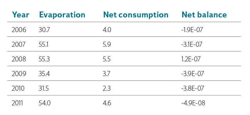
Blue water footprint values vary greatly depending on the approach used to determine water consumption (Fig. 1 and 2). The highest value is the blue water footprint when only considering water consumption in the form of evaporation (“gross consumption”). Both remaining approaches significantly reduce the water footprint value, even to negative values. Any negative value indicates that more water is flowing out of the reservoir than is flowing in through watercourses. Figure 1 shows that when considering evaporation only, the behaviour of volumetric water footprint values is characterized by seasonal performance, with peaks in summer and lows in winter. Conversely, water footprint values calculated using both “net consumption” (Fig. 1) and “net balance” (Fig. 2) do not show such seasonality. However, in the case of “net consumption” calculation, it should be noted that in this study only an indicative calculation of the evapotranspiration has been made to verify the principles of the method and the data are not entirely accurate. Nevertheless, this method of “suppression” of seasonality is already based on the principle of the method itself. For “net balance” calculation, the behaviour of monthly water footprint values is pre-determined by the characteristic behaviour of precipitation and temperature values during the year. As shown in Fig. 2, the water footprint determined through the “net balance” approach varies around 0, i.e. the precipitation reaching the water surface compensates for the evaporation from the surface. Table 1 presents volumetric water footprint values in yearly steps. Here, too, there is considerable variation in the values.
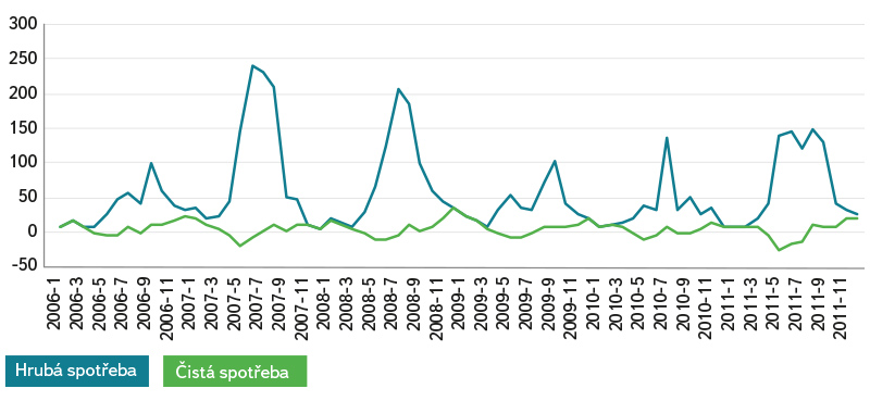
Fig. 1. Blue water footprint of Orlík HPS electricity – the methods of gross consumption and net consumption
Table 1. Volumetric water footprint values at Orlík HPS in yearly steps [m3·MWh-1]
The “gross consumption” method, which only considers evaporation, is the simplest approach; its main shortcoming, however, is suppressing the systemic approach to determining the use of water in what is termed “hydroelectric power generation system”. Looking at the reservoir as a component of the electricity generation system, there are several inputs into this system. Similarly, water “leaves” the system in the form of several outputs. Reservoir system inputs include: water courses flowing into the reservoir; sub-surface and, where appropriate, surface inflow from the reservoir surroundings, springs within the surface area of the flooded area; and precipitation reaching the water surface of the flooded area. Internal springs and the sub-surface/surface tributaries can usually be neglected due to their size and the fact that this water would reach the water course even without the existence of a reservoir. Outputs from a reservoir involve water that flows out of the reservoir, water that is extracted from the reservoir, and the water lost (whether through evaporation, seepage, or other means). Water collected from the reservoir can be neglected too, because it has no connection with the generation of electricity at the HPS (i.e., unless the station is located on a collection pipeline).
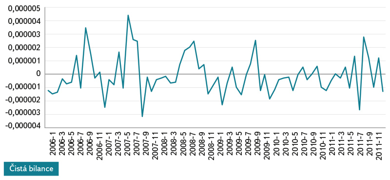
Fig. 2. Blue water footprint of Orlík HPS electricity – the net balance method
The calculation using the “net consumption” method is currently a frequently used approach [1] and assumes that there would be evaporation from the surface area of the reservoir even without the existence of the reservoir. The actual consumption is therefore equal only to the difference between potential evapotranspiration from the surface area of the flooded area of the reservoir and evaporation from its water surface. The application of this approach faces two major issues. First, any calculation of evapotranspiration will only be an estimate of this value. This is due to model approaches to determining actual evapotranspiration since any model is more or less just a precise simplification of reality. Above all, however, it is difficult to estimate at present what the structure of the surfaces in the flooded area would be. The second issue is a fundamental problem. Let us try to apply the principle of the “net consumption” approach to a factory, for example. The factory produces a product using Technology A that consumes 5 m3 per unit of produce. It undergoes a process of refurbishment and, after the modernization of its operations; the same factory is using Technology B that consumes only 3 m3 per unit of produce. Three conclusions can be drawn from this example. The water footprint of the product after factory refurbishment is 3 m3. The process has reduced the water footprint of the product by 2 m3. The total water footprint of factory’s produce has changed by (3× the number of products produced after the refurbishment) – (5× the number of products produced before the refurbishment).
It is possible to look at the given situation from another point of view as well. Prior to the construction of the reservoir, there was no HPS at the site, and all the evaporation from the flooded area of the current HPS was attributed (allocated) to the products that were produced in the area. For example, even if there was a power station on a weir in the area, then evaporation allocated to it would not be that from the surface area of the drainage basin, but only that from the weir pool. By building the reservoir, the use of the area has changed and the area produces other goods, such as electricity, raw water, protection from floods, and recreation.
The practical application of the “net consumption” approach is also problematic. Blue water footprint refers to the amount of water that is “consumed” when producing any goods (i.e., generating electricity in this case). Should long-term inflow to the reservoir be, for example, 1 million m3, long-term evaporation 2 million m3, and previous evapotranspiration (from the former surface before the reservoir was built) 1.2 million m3, then the water footprint would be 0.8 million m3. Should the reservoir be located in an arid region almost without precipitation, then it would actually be empty and nothing would be flowing out of it because losses of water from the system through evaporation would be higher than the input into the system in the form of inflowing water. The proposed “net consumption” approach is thus rather an example of inappropriate or special-purpose application, which is unfortunately an issue associated not only with water footprint but, generally with footprint methodologies [21].
In terms of methodology, the “net balance” approach appears to be the one most appropriate to address water footprint studies associated with the use of water in a reservoir. It includes losses of water from the system through evaporation as well as system “gain”, i.e., the input entering the system in the form of precipitation. However, even this is not completely clean in a methodical way. As Bakken et al. [4] point out, according to water footprint methodology [6], the water footprint value ranges from 0 to positive infinity.
When conducting water footprint studies associated with a reservoir, it is not appropriate to limit the inputs and outputs to only evaporation from the water surface and precipitation reaching the water surface; rather, it is appropriate to generalize the solution to apply to all inputs and outputs described above, even if, in a particular situation, individual input and output values can be considered as zero or negligible. In particular, losses via subsoil and surface inflow can both play a significant role in the overall reservoir balance under certain conditions. Factors that can cause a reservoir to stop working may not only involve errors when designing the reservoir and loss of water to the subsoil [22]. If a reservoir is situated in a level landscape and the surrounding soil has high permeability, the suction forces of the forest stands around the reservoir can affect the total losses of water from the reservoir with a high evapotranspiration capacity. In contrast, if there is very little permeable subsoil and minimum plant cover around the reservoir (which typically involves rocky surroundings of reservoirs), most precipitation from this area will flow directly into the reservoir. In both cases described above, it would be appropriate either to extend equations (1) and (5) to include terms expressing the influence of the surrounding area of the reservoir, or to consider some sort of an effective area of the reservoir. Any determination of such an effective area of the reservoir is not methodically developed at the moment. Hogeboom et al. [23], in their global study, only considered losses through evaporation (the “gross consumption” method); based on the theoretical average degree to which the reservoir can be filled and an idealized valley shape, this suggests using 56.25% of the maximum reservoir surface area as a reservoir surface area value for calculating losses through evaporation. For use with the “net balance” method, this value is rather underestimated.
Robescu and Bondrea [24] calculated the water footprint associated with the construction of the dam for the Vidraru HPS to be 19.7 million m3, with the dam volume being 480,000 m3 (i.e., 41 m3 per m3 of the concrete dam). Using this information and the volume of Orlík hydraulic structure of about 1.1 million m3, the water footprint of Orlík dam is 45.1 million m3, or (considering 100 years of service life) 4.51 million m3 per year. The calculated annual evaporation from Orlík reservoir is 15.5 to 17.1 m3 in individual years. Subsequently, converting it to a unit of electricity generated, it is 0.26 to 3.09 m3·MWh-1 in monthly steps, and 0.81 to 1.51 m3·MWh-1 in yearly steps. These are not negligible values, particularly when the “net balance” method is applied.
In the completed study, all inputs and outputs of the reservoir system were allocated to electricity generation. Orlík reservoir, however, is not just for generating power, but (like most of the reservoirs around the world) it is a multi-purpose facility [25]. In addition to electricity generation, it provides environmental functions (improved flow), flood protection, water collection, navigation, fishing, sport, and recreation. Therefore, the total water use should be redistributed (allocated) to all these uses, which will reduce the values of the water footprint determined for electricity generation. However, research on allocation methods for individual water uses is still very limited, and even studies that have included allocations for different uses in water footprint calculations use different methods [1, 26]. Different allocation methods can be used in the settings of the Czech Republic; specification through the economic value of individual uses provided by reservoirs is perhaps the most universal way. While expressing the economic value of both the electricity generated and the raw water collected is relatively easy due to the existence of a price, expressing the value of other uses is a task suitable for economists. It should also be noted that global research (especially in areas with limited water resources) also addresses the opposite role, i.e. how to use the water footprint to allocate water found in the reservoir as efficiently as possible for each use in order to achieve maximum benefits [27].
LCA water footprint
Calculation of regionalized values of the characterization factors for both models selected is identical, in principle; it differs only in different reference values, including the water needed for the ecosystems in the AWARE model and limiting the CFAWARE values to an interval of 0.1; 100. The characterization factors for both models have a relatively similar behaviour in individual months, although the variability of the values is very large (Fig. 3). The values of the characterization factor of CFfwua range between 0.9 and 12.9, with 5.9 being the average. The values of the characterization factor of CFAWARE even range between 0.16 and 15.8, with 2.3 being the average.
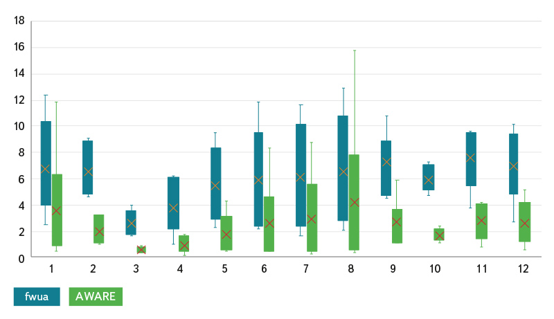
Fig. 3. The values of regionalized characterization factors
From the terminological aspect, the water footprint established by these two models represents a value of water scarcity footprint. Figures 4 to 6 show LCA water footprint behaviour in monthly steps by both characterization models, and comparison with the behaviour of the volumetric water footprint. In general, in the case of Orlík HPS, the two LCA models reduce the variance of values compared with volumetric water footprint. This statement does not apply only to the fwua characterization model applied to the use of water established through the “net balance” approach, where it rather highlights the maximum values (Fig. 6). The graphs charts show that the variance of the monthly values is very large. Table 2 shows the values in yearly steps and here, too, there is a significant variation in the water footprint values.
Table 2. LCA water footprint values of Orlík HPS in yearly steps [m3·MWh-1]
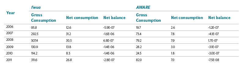
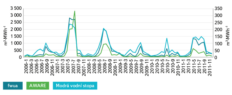
Fig. 4. LCA and volumetric water footprint – gross consumption
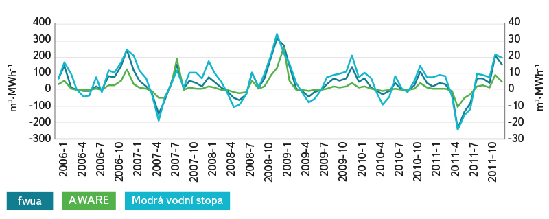
Fig. 5. LCA and volumetric water footprint – net consumption
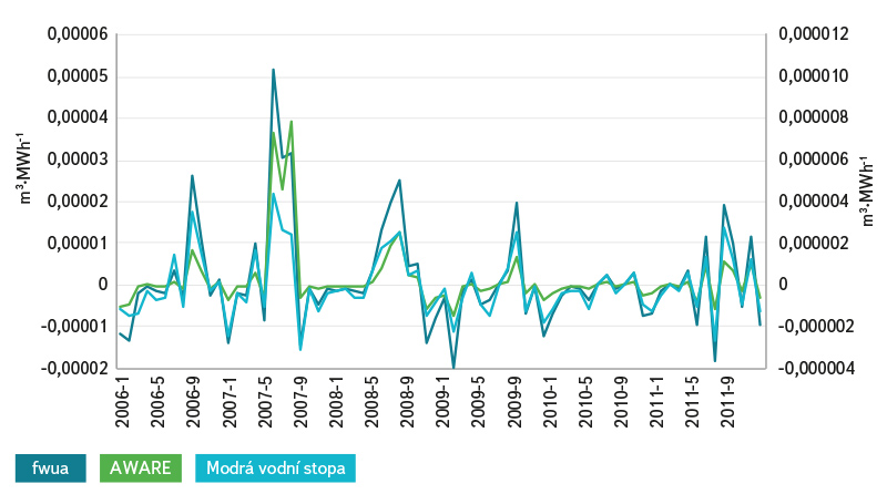
Fig. 6. LCA and volumetric water footprint – net balance
LCA studies are mutually problematic for comparison because they are usually based on different assumptions and applications of simplification as well as characterization models. Using the fwua characterization model and using the same regionalization method, an LCA water footprint was established for 32 heat-generating plants and coal-fired power stations, while no processes other than the electricity generation itself were considered in these operations. The LCA water footprint of these operations ranged between 1.3 and 12.8 m3·MWh-1 [13]. Another LCA water footprint study is one conducted for Temelín and Dukovany nuclear power stations (NPS), where a regionalized fwua characterization model was used and only evaporation was considered to determine the loss from reservoirs [28]. LCA water footprint values in yearly steps ranged from 6.1 to 7.7 m3·MWh-1 for Temelín NPS and between 15.0 and 16.5 m3·MWh-1 for Dukovany NPS. The AWARE model was also applied to these two power stations; again, considering only evaporation [29], and LCA water footprint values in yearly steps were between 1.3 and 1.6 m3·MWh-1 for Temelín NPS, and between 3.2 and 3.5 m3·MWh-1 for Dukovany NPS.
Conclusion
The water footprint study for Orlík HPS has shown some important facts to bear in mind when carrying out future water footprint studies. Of these, the choice of how water use is calculated is clearly the most important. The “gross consumption” method only considers evaporation from the reservoir, and is therefore clearly dependent on the course of meteorological variables during the year. At the same time, it also exhibits the highest water footprint values. The “net consumption” method subtracts the value of drainage basin surface area evaporation (before construction of the reservoir) from water surface evaporation. Although this method has been widely used in recent years to calculate an HPS water footprint, its accuracy is debatable. The “net balance” method can be recommended as an appropriate approach.
The issue of allocation is another important aspect that affects the water footprint value relative to the unit of electricity generated. In the Czech Republic, virtually all reservoirs provide multiple benefits, so applying all of the water use to only one benefit (e.g. electricity generation) is methodically incorrect. However, the procedures of allocating the use of water to individual benefits provided by the reservoir are not yet standardized.
The last important aspect is the question of neglecting the construction and decommissioning stages of a hydraulic structure. Although these stages of the life cycle of an HPS are usually neglected in global studies, on the grounds that they become “dissolved” to negligible values over the life cycle, an indicative calculation based on literature data has shown that, for Orlík HPS, these may not be negligible numbers, especially when using the “net balance” method and, to some extent, even when using the “net consumption” method.
