ABSTRACT
The main objective of the article was to optimize the facilities used to distribute flows in inlet galleries, which are used not only in water treatment plants, but also in wastewater treatment plants (WWTP). While working in the field of WWTP, it was found that there are no optimized facilities in the Czech Republic or globally for uniform distribution of flows to any number of inlet branches into reservoirs of the same flow rate. Currently, in most unregulated facilities, there are significant differences between the various inlet branches to the reservoirs. In regulated facilities, the outlets must be regulated at each change in flow rate and, for changes in the number of inlets to the reservoir (e.g., due to reservoir shutdown), each outlet must be manually adjusted (e.g., using a sluice gate) so that all inlets to reservoirs have the same flow rate. In more modern cases, the sluice is equipped with an electric motor for changing the position and a probe sensing the level. The central unit then calculates the flow rate in the individual reservoir inlets and adjusts the position of the sluice gates so that the same flow rate is achieved everywhere. The objective of the research was to optimize the distribution facility so that the inlets to the reservoirs reach similar values for the flow rate when both the inflow to the distribution facility and the number of inlet branches to the reservoirs are changed, without significant regulation at the distribution facility. In order to make the research easily applicable to as many distribution facility as possible, the most commonly used flow distribution facilities (fountain spillway, flume with outlets fitted with a sluice gate and probe for level monitoring, etc.) were selected to address the issue. Different flow conditions were simulated on the selected facilities (in different variants and shapes); after their analysis the facilities were optimized in order to achieve the most similar flows at the inlets to the individual reservoirs.
INTRODUCTION
This article presents a CFD (Computational Fluid Dynamics) model of a selected facility distributing flows at a WWTP. This facility was chosen because it is one of the most used at the WWTP. The facility divides the flow from the aeration tanks into four reservoirs. Observations during operation showed that the flow is not evenly distributed – there are significant differences between the inlets to individual reservoirs.
Single-phase flow with pure water was simulated on the model. Air bubbles and sludge flocs were not included. The sensitivity analysis showed some influence of the inflow turbulence characteristics on the final results. Since the inflow comes directly from the aeration tank with fine bubble aeration, the determination of turbulence is very difficult. All results are from the uncalibrated model.
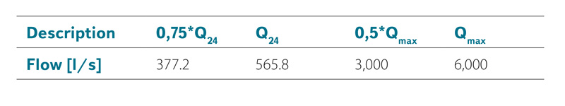
Since the flows to be simulated were not explicitly specified, the following flows were chosen:
Tab. 1. Simulated flows
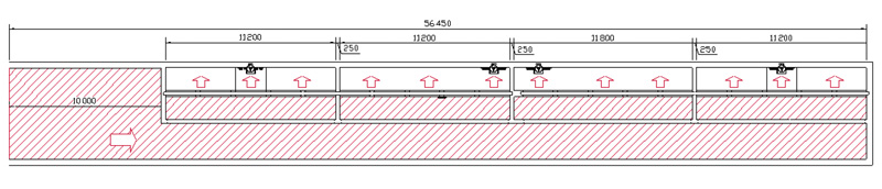
The geometry of the model was set according to the available drawings of the most used facilities at the WWTP. A 10 m long section of the aeration tank was simulated together with the flow distribution structure in order to achieve a fully developed flow field at the beginning of the flow distribution structure [1].
 Fig. 1. CFD model – cross section – simulated part marked in red
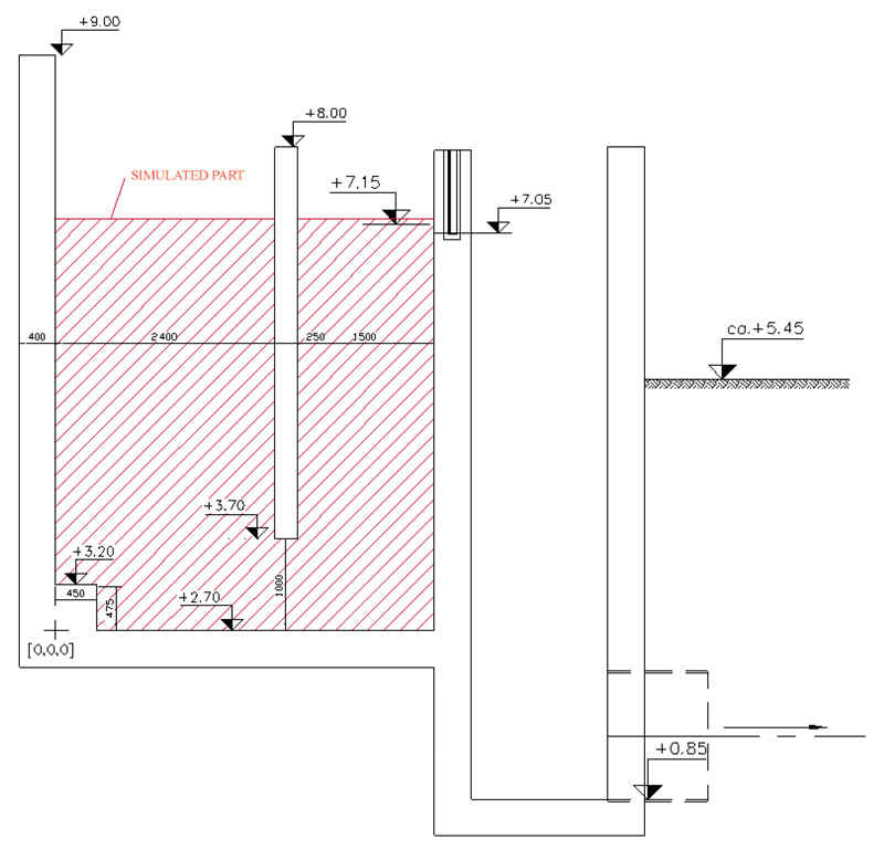
Fig. 2. CFD model – floor plan – simulated part marked in red
METHODOLOGY
Before any simulation, it is important to have a general understanding of how the structure works and to establish the most important phenomena taking place there. Flow distribution facilities are usually based on outlet openings. The overflow velocity of the outlet opening is determined by the hydraulic elevation in front of it. Therefore, if openings of the same length have the same overflow height, the flow rate must be the same. However, even a small change in water level causes large differences between the flows.
And that is the problem with this facility. The channel, which distributes the flow to the four outlet openings, is quite long and a backflow is formed along it. The water level in the facility will therefore not be constant. The openings in the bed that drain the water into the reservoirs are relatively large and therefore do not contribute to an even distribution of the flow.
Water levels at the facility
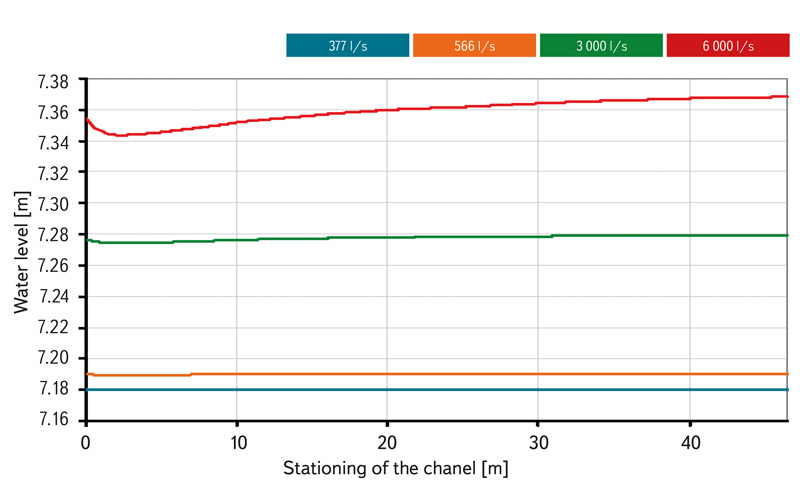
Four different simulations of the distribution facility with different flow rates were performed. The results show that the above considerations are correct. At the beginning of the channel, the water level drops. As the water flows from the aeration tank into the narrow channel of the distribution facility, the velocity gradient increases and therefore the water level must drop. Further along the channel, part of the water flows through side openings into the reservoirs, the flow rate decreases and the water level increases [2].
The model shows this at all flow rates. At low flow rates (377 and 566 l/s) the difference is so small that this effect is only theoretical and in reality the more significant difference in water level is caused by other factors (waves, wind). However, at high flow rates (3,000, 6,000 l/s), this effect is quite significant. This is shown in the following figures (Fig. 3–7). The colour scale shows the difference between the constant level approximation and the simulated water level in metres.
All described effects can be seen even better in Fig. 7. The height of the water level is shown in metres.
Fig. 3. Simulated water level difference Q = 377 l/s
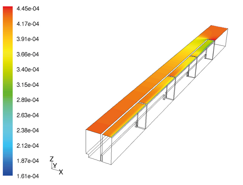
Fig. 4. Simulated water level difference Q = 566 l/s
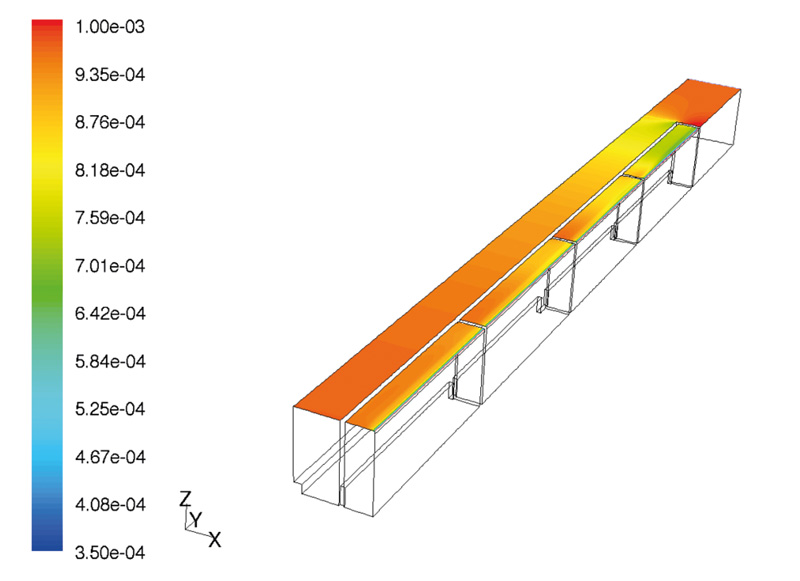
Fig. 5. Simulated water level difference Q = 3,000 l/s
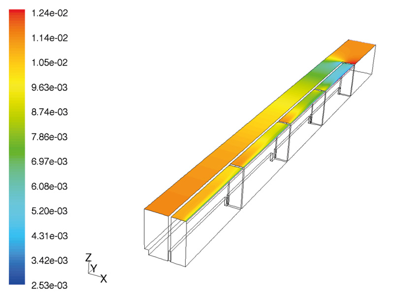
Fig. 6. Simulated water level difference Q = 6,000 l/s
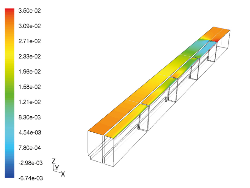
Fig. 7. Simulated water level in the flow distribution object
RESULTS
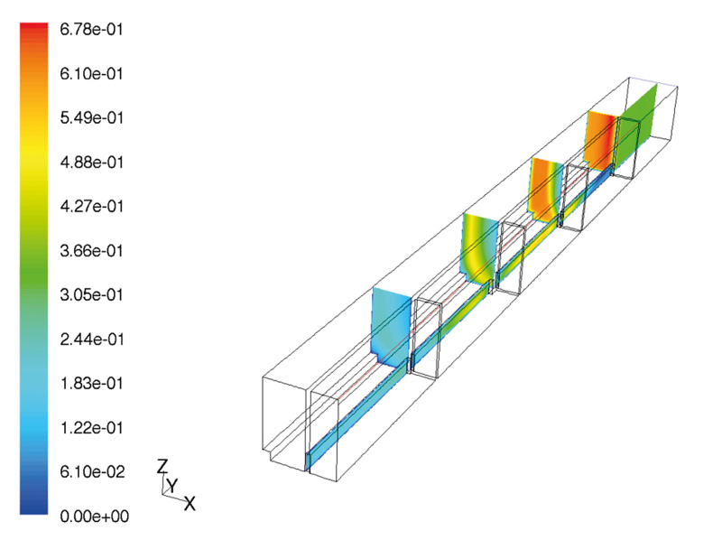
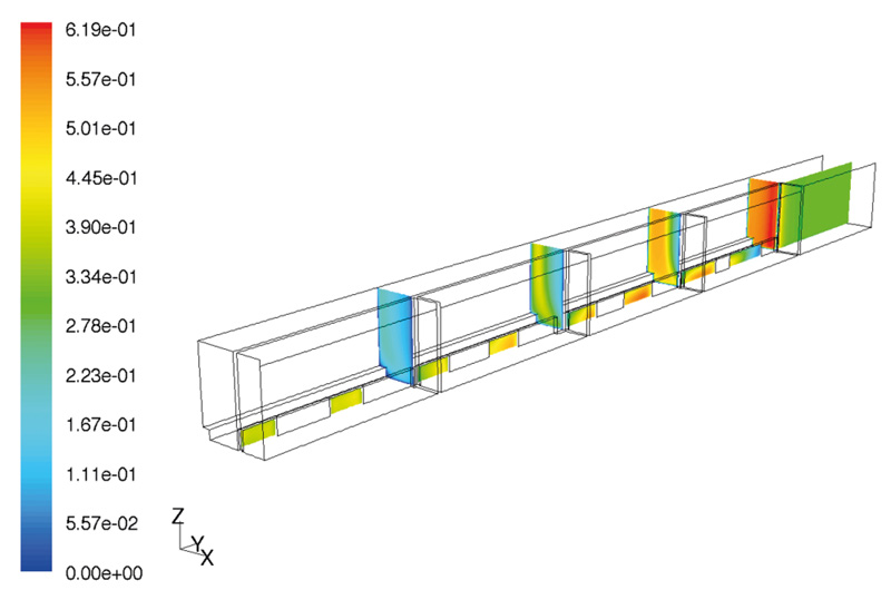
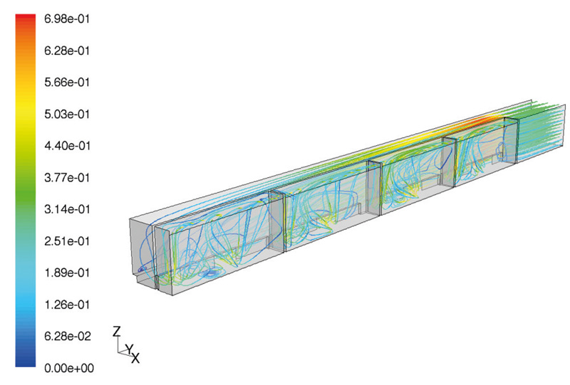
Fig. 8–11 show the contours of the simulated flow velocities in the channel cross-sections and in the openings, which can give some idea of the general flow pattern.
At the beginning of the channel, the flow narrows quite significantly. It means that the first half of the first opening is not fully utilized hydraulically. This is again more important under high flow conditions. This effect could actually be less significant than in the model because there is high turbulence in the aeration tank, which is difficult to assess in the model.
The colours represent the overall velocity. Therefore, the velocity in the last opening is the lowest. The “y” component of the velocity is quite significant in the first three openings [3].
Fig. 8. Flow velocity contours Q = 377 l/s

Fig. 9. Flow velocity contours Q = 566 l/s
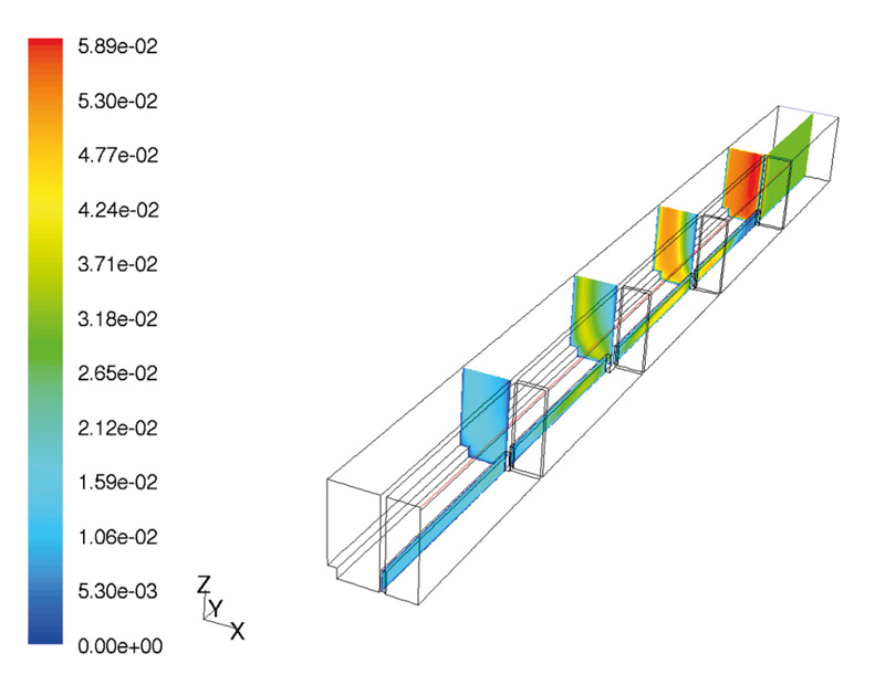
Fig. 10. Flow velocity contours Q = 3,000 l/s
Fig. 11. Flow velocity contours Q = 6,000 l/s
Flow distribution
Tab. 2 and Fig. 12 show the flow distribution under different flow conditions. Since no measured data were available, the model could not be calibrated. The sensitivity of the flows to the overflow height was adjusted only according to the theoretical flow curve. Preliminary results showed a similar distribution of flow under all flow conditions; however, at low flows the overflows were found to be too sensitive to overflow height. The final results after appropriate adjustment of this sensitivity are shown in Tab. 2.
Tab. 2. Flow distribution
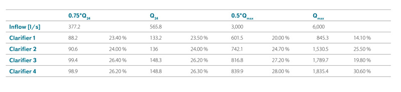
Fig. 12. Flow distribution
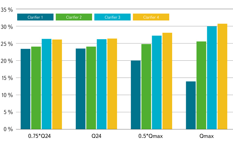
The results show that the flow distribution is fairly evenly distributed at low values; however, with increasing flow, the unevenness of the distribution increases, which is caused by the differences in the water level described above [4].
DISCUSSION
Since the results showed that the flow distribution is not dependent on the flow itself, it was proposed to solve the problem by adjusting the lengths of the overflows.
The introduction of baffles across the channel does not seem like a good idea either. The channel itself is quite narrow and introducing any major obstructions into it would reduce its hydraulic capacity and rather make the problem worse.
The best solution is probably adjusting the size of the openings at the channel bed to distribute the flow. Smaller openings at the end of the channel will cause a hydraulic loss that will compensate for the higher water level at high flow rates. At low flow rates, the hydraulic loss will be small and the flow distribution will not be affected.
Setting the size of the lower openings
Several simulations were performed to find the best possible combination of opening sizes. The optimization was based on the maximum flow rate (6,000 l/s) and a flow rate of 566 l/s was used to confirm the good performance of the design at low flow rate.
The simulations were performed iteratively. First, the size of the openings was reduced to half the original size. The original openings were very large (velocity 0.136 m/s at maximum flow rate), and although their size was halved, they did not cause much energy loss. The flow through the modified structure was simulated and the flow rates into the individual reservoirs were obtained.
Optimization process
Tab. 3 and Fig. 13 show the simulation results of the above versions and show the iteration process.
Tab. 3. Comparison of the different phases of the iterative process (Qmax)
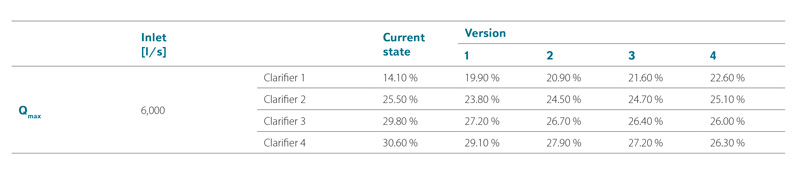
Fig. 13. Example of iterative process

Proposed improvement
The proposed improvement is shown in Fig. 14. The red hatched areas show the placement of the plates that close the parts of the openings. In the simulations, these baffles were placed on the side of the channel and were aligned with the channel wall.
Fig. 14. Final dimensions of the proposed openings
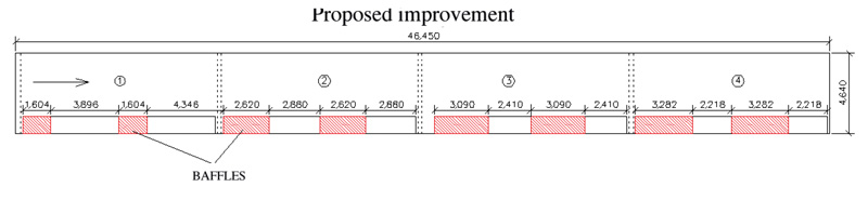
Fig. 15. Velocity contours of the flow pattern Q = 6,000 l/s
Function principle
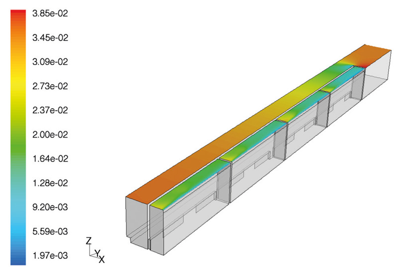
The following figure (Fig. 16) shows the function of the baffles in the lower openings. Although the water level rises along the channel, the water levels in the still chambers are almost equal. The difference between the water levels in the channel and in the still chamber is due to hydraulic losses caused by the baffles. The colours in the figure show the difference between the approximate constant water level and the calculated level.
Fig. 16. The water level in the distribution object
CONCLUSION
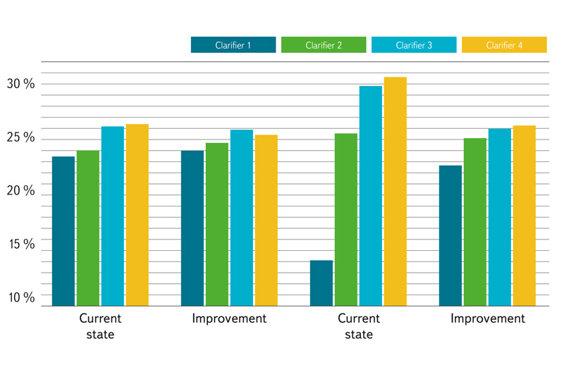
The following table and diagram (Tab. 4, Fig. 17) show a comparison of the simulation results for the current state and the final proposed improvement. For improvement, only the maximum flow (Qmax) and the mean daily flow (Q24) have been simulated so far. It can be seen from the results table that the proposed state of the distribution facility meets the conditions for an even distribution of flows, and the objectives of the research have thus been fulfilled. Considering the fact that the selected distribution facility is commonly used in the field, the results of the research can be easily applied in practice, namely to a larger number of WWTP.
Tab. 4. Comparison of the current situation and proposed improvements
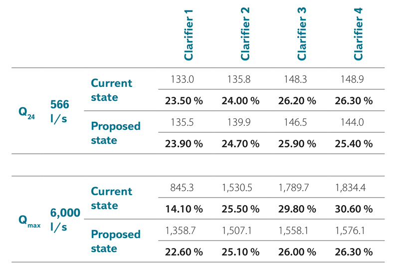
Fig. 17. Comparison of the current situation and proposed improvements
Other possible improvements
This improvement shows that it is possible to reduce the problem of uneven flow distribution by introducing baffles into the openings, the installation of which is quick, simple, and without the need for building modifications. Further attention in possible follow-up research should be paid to the shape of the baffles.
It cannot be ruled out that some sediments could accumulate in the quiet zones behind these baffles and especially in the corners (Fig. 18), which could cause a problem with sediment clogging the inlet branches into the reservoirs in the future. Clogging with sediment will most probably affect the hydraulics of the distribution facility so that the uneven flow distribution will occur again.
Fig. 18. Sediment is likely to accumulate in dead zones in the corners
Acknowledgements
This article was supported by grant 3600.54.10/2021 “3D modelling of selected
variants of flow distribution in inlet galleries”.
The Czech version of this article was peer-reviewed, the English version was translated from the Czech original by Environmental Translation Ltd.
