

ABSTRACT
This article presents proposed approaches for assessing changes in the status of surface waters, i.e. progress towards achieving good status as a result of the measures implemented. The approaches are based on newly recalculated assessments for individual profiles, indicators and three-year periods, using the most recently approved characteristic values and limits. In addition to the overall result (good/non-compliant status), each profile, indicator, and three-year period is assigned a non-compliance index, which is the ratio of the characteristic value to the good status limit. The next step is to classify the non-compliance index into categories that represent either the extent to which the limit is exceeded or, conversely (for good status categories), proximity to the limit. When comparing results for individual three-year periods, it is necessary to select only those profiles with measurements for the entire assessment period to ensure the comparison is reliable.
The approach was also applied to ten of the most problematic indicators of ecological and chemical status/potential (with the exception of biological quality elements, which were not addressed by the project).
The results showed that concentrations of nitrate and ammoniacal nitrogen, fluoranthene, alachlor metabolites and AOX are decreasing and that good status is being achieved more frequently; concentrations are also decreasing in profiles where the non-compliance index is high. Concentrations of BOD5, metolachlor and its metabolites, and EDTA are generally stable; concentrations of total phosphorus and phosphate phosphorus are stable or even slowly increasing, while high concentrations show no improvement either.
INTRODUCTION
An important component of River Basin Management Plans (RBMP) under the Water Framework Directive (WFD) [1] is the assessment of the status of water bodies. The objective of RBMPs is to achieve good ecological status (or good ecological potential, where applicable) and good chemical status of surface waters. For the purposes of RBMPs, the status of surface waters is assessed once every six years. However, pursuant to Section 4 of Czech Decree No. 98/2011 Coll., on the method for assessing the status of surface water bodies, the method for assessing the ecological potential of heavily modified and artificial surface water bodies, and the requirements for programmes for the monitoring and assessment of the status of surface waters, as amended [2], the status of surface water bodies is evaluated every three years. For the purposes of RBMPs, the results from the later of these two three-year assessment periods are used. Thus, during the third RBMP cycle, surface water status was evaluated for both the 2013–2015 and 2016–2018 assessment periods, with the RBMP being based primarily on the results for 2016–2018.
Although chemical status and ecological status/potential each comprise multiple quality elements or pollutants, for which the “one out, all out” principle applies (i.e. the overall status is determined by the lowest classification), the results are generally presented in aggregated form as a single ecological or chemical status for each water body. Since status assessments have been carried out since 2010, many changes have occurred over the past 16 years at both the European and national levels. These include changes in the delineation of water bodies, the selection of indicators, good status limits, assessment methodologies, and the indicators monitored. At the same time, measures to improve water status have also been implemented. As a result, it is very difficult to determine from the aggregated assessment results alone whether the situation is improving. The implementation of these measures is also very costly, making it essential to evaluate their effectiveness. This is important both for the institutions responsible for designing and implementing the measures and for the wider public. At the European level, there is now a consensus that, in order to assess progress towards achieving good status, ecological status assessments should be broken down at least into the individual quality elements: biological, hydromorphological, chemical (specific pollutants), and physicochemical. Similarly, chemical status assessments should distinguish between so-called ubiquitous substances and all other substances. For chemical status, the European Commission requires results to be reported using this classification to ensure comparability. However, experience has shown that even this level of classification is not sufficiently detailed.
Discussions at the European level have shown that it is very difficult to develop a single approach to assessing progress towards achieving good status that is suitable for all Member States. This is because both the frequency and timing of monitoring for individual indicators or pollutants, as well as the methods used to assess status, differ between countries. For example, some countries assess the status of selected chemical status indicators every year and use the most recent assessment. In contrast, other countries assess these indicators only in selected years. In the Czech Republic, chemical status is generally monitored annually, with the overall status being determined by the worst result recorded during the preceding three-year period. For general physicochemical indicators (e.g. nutrients, temperature, and oxygen), the assessment is based on the results for a three-year period. In the Czech Republic, this is usually the median value calculated from the previous three years (with maximum values also used for nitrate nitrogen and temperature). However, the assessment methods differ between individual countries. For example, both Austria and the Czech Republic assess nitrogen in surface waters as nitrate nitrogen, and the boundary between good and moderate ecological status is defined according to river type. The threshold values generally range from 3.0 to 4.0 mg/L (compared with 2.3–3.8 mg/L in the Czech Republic). However, in Austria, the assessment is based on the 90th percentile of data collected over the entire calendar year, with the final status corresponding to the worst annual result recorded during the entire six-year assessment period [3]. In Hungary, total inorganic nitrogen is assessed, with annual arithmetic mean threshold values ranging from 1.4 to 5.0 mg/L. However, if the phytobenthos or phytoplankton is classified as being in good status, the result for total inorganic nitrogen is disregarded. For status reporting, a six-year arithmetic mean is calculated from all annual mean values. However, if nitrogen concentrations show a clear upward trend during the last three years of the assessment cycle, only data from those three years are used [4]. In France, nitrates are assessed, with a single good status threshold of 50 mg/L (ca. 11.3 mg/L nitrate nitrogen) applying to all surface waters. As in Austria, the annual 90th percentile is used. However, as in the Czech Republic, the final status is based on the results from the last three years of the monitoring cycle, calculated as the 90th percentile [5]. This brief overview clearly demonstrates that assessment methodologies vary considerably. Consequently, attempts to establish a common European methodology have generally resulted in the adoption of the lowest common denominator [6]. Although this approach may facilitate comparisons between countries, its value for assessing progress is considerably limited.
For these reasons, the methodology presented in this paper was developed to assess progress towards achieving good surface water status. The methodology was developed as part of Research Project No. SS02030027, Water Systems and Water Management in the Czech Republic under Climate Change. Although it is based on the fundamental European principles [6], it has been adapted to the data and assessment procedures used in the Czech Republic.
METHODOLOGY AND DATA USED
Before the most appropriate methodology was selected, different approaches were tested over a relatively long period. The most common approach was to compare water bodies achieving good status with those failing to achieve good status (Fig. 1), with the map showing changes in ecological status/potential between two RBMP cycles [7].
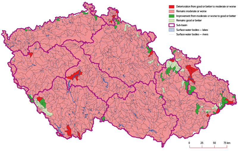
Fig. 1. Changes in the ecological status or ecological potential of surface water bodies between the periods 2016–2018 and 2022–2024
Ecological status/potential was selected for this comparison because it is the simplest parameter to compare. Both three-year assessment periods were evaluated using the same methodology, and the ecological status of almost all water bodies was assessed (i.e. there were very few unassessed water bodies). The map clearly shows that only a small number of changes in ecological status/potential occurred, including both improvements (green water bodies) and deteriorations (red water bodies). During the 2022–2024 assessment period, the status of 18.3 % of water bodies improved. However, an improvement did not necessarily mean that good status had been achieved, as improvements also included changes from bad to poor status and from poor to moderate status. By contrast, the status of 14.7 % of water bodies deteriorated, while 3.4 % remained in good status and 63.6 % remained in less than good status. However, this method of comparison provides no information on the reasons for the observed changes in status.
Changes in chemical status were illustrated in the same way (Fig. 2). Since some water bodies were not monitored during one or both three-year assessment periods (or because too few measurements were available), considerably more status categories were required. These additional categories cannot simply be ignored. Alternatively, they could all be grouped together as unknown, but this would not accurately reflect the underlying data. Consequently, the overall results are both less informative and more difficult to interpret. An improvement to good status was recorded for 10.6 % of water bodies, while 10.8 % deteriorated. A further 18.5 % remained in good status, 37.3 % continued to fail to achieve good status, and 22.8 % could not be assessed during at least one of the two three-year assessment periods (most recently in 2022–2024).
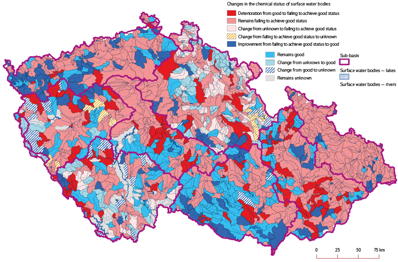
Fig. 2. Changes in the chemical status of surface water bodies between the periods 2016–2018 and 2022–2024
Note: Minor final changes for 2022–2024 are not included in the maps or percentages.
To assess changes in ecological and chemical status, it is necessary to examine the individual indicators and, where appropriate, the individual quality elements. The first question is which indicators and quality elements should be considered. Excluding the hydromorphological quality element, which serves only as a supporting element, there are 5 biological quality elements, 10 general physicochemical indicators, and 137 specific and priority pollutants. However, not all quality elements and indicators are equally important in terms of failing to achieve good status. This article does not examine the biological quality elements, although they are highly significant and were responsible for 76.3 % of water bodies failing to achieve good ecological status or ecological potential during the 2022–2024 assessment period. An even higher proportion (88.7 %) was attributable to the general physicochemical indicators. Ecological status also includes specific pollutants, which were responsible for 42 % of water bodies failing to achieve good status.
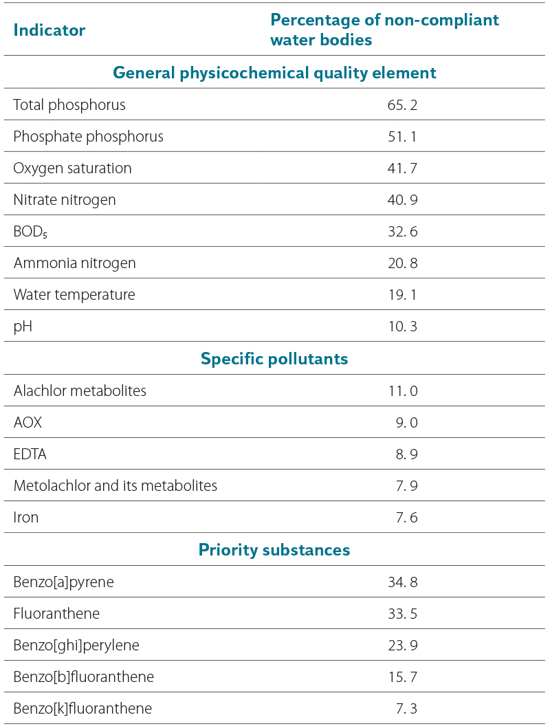
However, when individual indicators are considered, the number of those that are truly significant is much smaller (Tab. 1).
Tab. 1. Indicators that most often fail to achieve a good status in the three-year assessment 2022–2024
To assess trends in individual indicators, it is appropriate to compare successive three-year assessment periods. Assessment results are available for a total of five such periods, ranging from 2010–2012 to the most recent period, 2022–2024. The use of three-year periods reduces the influence of fluctuations in concentrations, which are mainly caused by changing hydrological conditions, including short-term droughts and, conversely, flood events. However, as already mentioned, the first three assessment periods were accompanied by substantial changes in the assessment methodology, such as the redelineation of surface water bodies, changes to the assessment procedures (including the definition of the boundaries between good and moderate ecological status and between good and failing to achieve good chemical status), and the gradual inclusion of additional priority substances and matrices in the assessment of chemical status. These factors, which prevent direct comparison of status assessment results, were recognised at the European level some time ago. However, another equally important change has still not received sufficient attention: the gradual expansion of the range of monitored indicators.
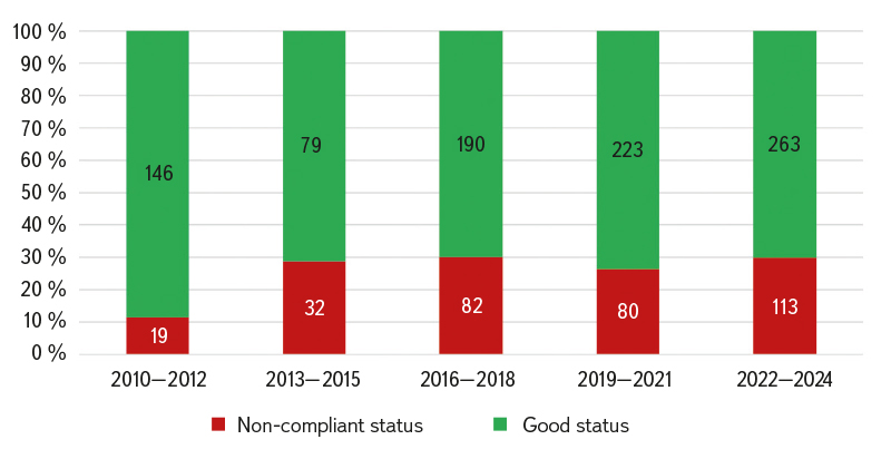
The progressive expansion of monitoring can be illustrated by ethylenediaminetetraacetic acid (EDTA), which is classified as a specific pollutant in the Czech Republic and was monitored and assessed at 165 monitoring sites during the first three-year assessment period and at 376 sites during the most recent period (Fig. 3).

Fig. 3. Assessment of ethylenediaminetetraacetic acid (EDTA) in individual three-year periods based on good status limits (numbers in the graph represent the number of water bodies)
However, when assessing trends in individual indicators in terms of progress towards achieving good status – and thus the effectiveness of the measures implemented – it is necessary to consider more than the status assessment results alone. Several key principles should therefore be followed:
- the assessment period should be as long as possible,
- results should be based on three-year assessment periods,
- the assessment should be based on the established methodologies and good status thresholds,
- only monitoring sites for which analytical data are available for the assessment periods should be included,
- the assessment should focus not only on the achievement of good status, but also on trends in decreasing or increasing concentrations.
Notes
The assessment period should begin only after the introduction of RBMPs. Otherwise, the analysis would measure general improvements in water quality rather than the effectiveness of measures implemented under the RBMPs. If data from the 1990s were used (provided they were of sufficient quality), the apparent improvement – at least for the conventional indicators – would naturally be much greater. However, such improvements would not be attributable to measures implemented under the RBMPs.
The current assessment methodologies and good status thresholds should be used. Where these thresholds have changed over time, the currently applicable thresholds should be applied, as they are generally more stringent. Nevertheless, a single approach cannot be applied to all indicators. For specific pollutants and priority substances, where annual mean concentrations are used and the status is determined by the worst annual result, the annual means are recalculated from the primary data for each three-year assessment period, and the resulting three-year mean values are compared. Where both a median and a maximum value, or a mean and a maximum value, are used for status classification, only the median or mean is suitable for comparing trends. Although we attempted to assess trends in maximum values, we found no method that produced meaningful and reliable results. Consequently, many priority substances cannot be assessed because they are classified solely on the basis of maximum values. This makes it necessary to use the primary data rather than relying solely on the status assessment results. Initially, only the first and the most recent three-year assessment periods were compared. However, it was ultimately found to be more appropriate to include all five three-year assessment periods.
Only monitoring sites for which water quality data are available throughout the entire assessment period can be used to assess trends. This addresses both changes in the delineation of water bodies (by including only monitoring sites that consistently represented a water body throughout the assessment period) and changes in the range of monitored indicators. Although this reduces the number of monitoring sites that can be assessed compared with the present day, it ensures that the results are comparable.
The final principle is equally important. Particularly for indicators with a high proportion of non-compliant results, it is important to assess not only whether good status has been achieved, but also whether concentrations are generally decreasing, remaining stable, or increasing. Calculating trends for individual monitoring sites is labour-intensive and, when based on linear trend analysis, is also relatively unreliable [8]. A simpler approach was therefore adopted by classifying the results according to the so-called non-compliance index, calculated as the ratio of the relevant characteristic value to the good status threshold. For all indicators, the following categories were used: ≤ 0.8; 0.8–1 (both representing good status); 1–1.5; 1.5–2; and > 2. Where a large number of monitoring sites failed to achieve good status and the non-compliance indices were also high, additional categories with higher non-compliance index thresholds (2, 3, and 4, or 2, 4, and 7) were introduced.
The following indicators were ultimately excluded from Tab. 1: oxygen saturation, water temperature, pH, iron, benzo[a]pyrene, ben-zo[ghi]perylene, benzo[b]fluoranthene, and benzo[k]fluoranthene. In most cases, the reason was that status assessment is based solely on maximum values. The exceptions were water temperature (for which the thresholds will probably need to be revised in response to climate change), iron (because it is not possible to distinguish reliably between naturally elevated concentrations and anthropogenic pollution), and benzo[a]pyrene, for which the environmental quality standard (the good status threshold) was, until recently, lower than the limit of quantification.
For the remaining indicators, the individual non-compliance index categories were calculated and compared across all three-year assessment periods. For the general physicochemical indicators, the analysis covered the period from 2010–2012 onwards; for fluoranthene and the specific pollutants, from 2013–2015 onwards (because substantially fewer monitoring sites were included in the first three-year assessment period); and for ethylenediaminetetraacetic acid (EDTA), from the third assessment period (2016–2018) onwards. The analysis included all representative monitoring sites of surface water bodies in the Czech Republic. The number of monitoring sites meeting the selection criteria varied considerably: 793–850 for the general physicochemical indicators, 310–343 for fluoranthene and the specific pollutants, and only 203 for ethylenediaminetetraacetic acid (EDTA).
RESULTS AND DISCUSSION
General physicochemical indicators
The results for the general physicochemical indicators differ considerably. For both nitrate nitrogen and ammoniacal nitrogen (Figs. 4–8), the concentrations show a declining trend, both across the individual non-compliance index categories and in terms of achieving good status. For nitrate nitrogen, the difference between the first and the most recent three-year assessment periods was 7.8 percentage points (Fig. 5), compared with 7.3 percentage points for ammoniacal nitrogen (Fig. 6). Ammoniacal nitrogen also showed a marked reduction in high concentrations, both in terms of the number of monitoring sites and their proportion (Fig. 7).
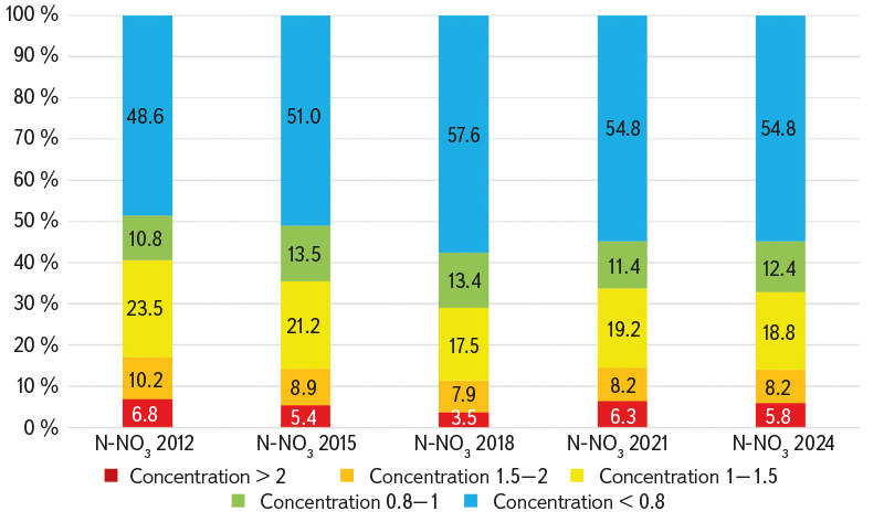
Fig. 4. Proportion of profiles by multiples of nitrate nitrogen concentrations relative to the limit in each three-year period
Note: The three-year periods are designated by their final year.
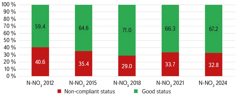
Fig. 5. Proportion of profiles by nitrate nitrogen limits in each three-year period
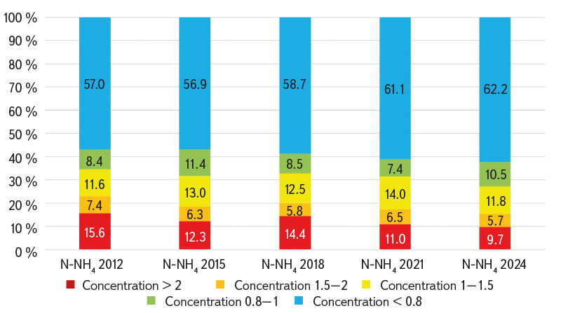
Fig. 6. Proportion of profiles by multiples of the ammoniacal nitrogen concentrations relative to the limit in each three-year period
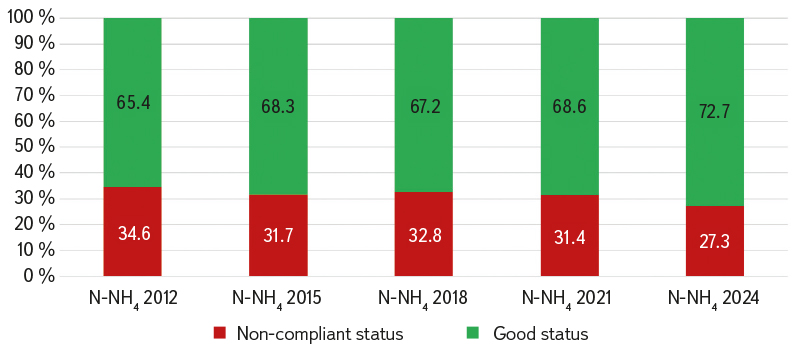
Fig. 7. Proportion of profiles by ammoniacal nitrogen limits in each three-year period
Fig. 8. Proportion of profiles by multiples of the ammoniacal nitrogen concentration relative to the limit in each three-year period – high concentrations (numbers in the graph in brackets represent the number of profiles)
The main difference between the two indicators lies in their trends across the individual three-year assessment periods. Nitrate nitrogen concentrations were lowest during the 2016–2018 assessment period, when the effects of a prolonged drought were apparent. Concentrations increased slightly during the following three-year period before declining again. This was probably because the principal source of nitrate nitrogen is diffuse agricultural pollution. During dry periods, nitrogen is not leached from the soil, although it is also taken up less readily by plants. It is released into surface waters only after precipitation increases again. Differences between the individual three-year assessment periods were less pronounced for ammoniacal nitrogen, which can probably be explained by the fact that its principal source is municipal wastewater rather than agriculture.
Although biochemical oxygen demand (BOD₅) showed a smaller improvement in status than the nitrogen forms (Fig. 10), it exhibited equally marked reductions in high concentrations (Fig. 9). It should be noted that the greatest reductions in BOD₅ concentrations occurred during the period 1990–2010, and that improvements have been more gradual since then.
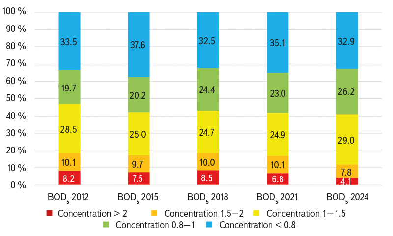
Fig. 9. Proportion of profiles by multiples of the biochemical oxygen demand concentrations relative to the limit in each three-year period
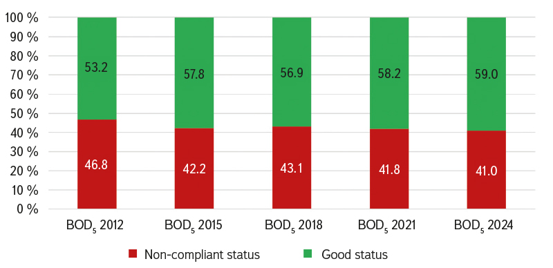
Fig. 10. Proportion of profiles by biochemical oxygen demand limits in each three-year period
The remaining general physicochemical indicators are total phosphorus and orthophosphate phosphorus (Figs. 11–13). Unfortunately, unlike the previous indicators, they show virtually no improvement, with only minimal differences between the individual three-year assessment periods. Compared with total phosphorus, phosphate phosphorus exhibits only slightly lower non-compliance indices (Fig. 13) and a somewhat higher proportion of monitoring sites achieving good status.
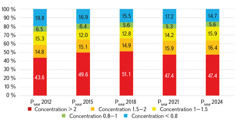
Fig. 11. Proportion of profiles by multiples of the total phosphorus concentrations relative to the limit in each three-year period
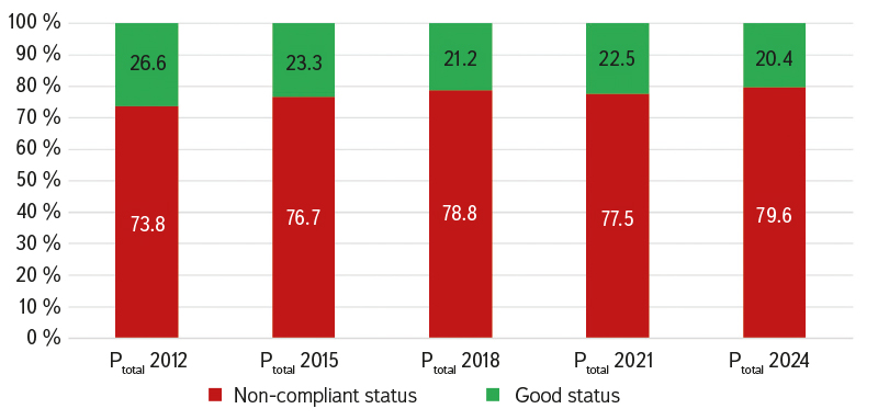
Fig. 12. Proportion of profiles by total phosphorus limits in each three-year period
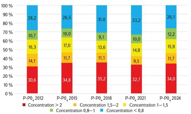
Fig. 13. Proportion of profiles by multiples of the phosphate phosphorus concentrations relative to the limit in each three-year period
Fluoranthene and specific pollutants
Unlike the general physicochemical indicators, for which gradual improvement was observed only for nitrate nitrogen and ammoniacal nitrogen, fluoranthene, alachlor metabolites, and adsorbable organically bound halogens (AOX) showed marked improvement. For fluoranthene, substantial reductions in concentrations can be observed in all three types of graphs (Figs. 14–16). The proportion of monitoring sites achieving good status increased by 13.4 percentage points (Fig. 15), while the proportion with concentrations exceeding a non-compliance index of 7 decreased markedly from 5.5 % of all monitored sites to just 1.5 % (Fig. 16). In addition, the decline was gradual, with no evidence of pronounced fluctuations.
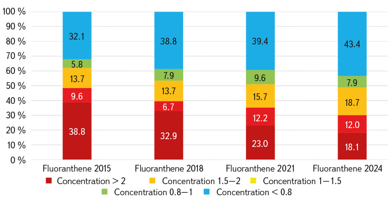
Fig. 14. Proportion of profiles by multiples of fluoranthene concentrations relative to the limit in each three-year period
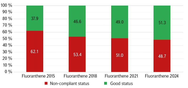
Fig. 15. Proportion of profiles by fluoranthene limits in each three-year period
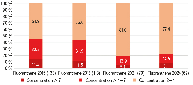
Fig. 16. Proportion of profiles by multiples of fluoranthene concentrations relative to the limit in each three-year period – high concentrations (numbers in the graph in brackets represent the number of profiles)
A similar pattern was observed for alachlor metabolites. The proportion of monitoring sites achieving good status increased by 10.6 percentage points (Fig. 17), while the proportion with concentrations exceeding a non-compliance index of 4 declined markedly from 4.8 % of all monitored sites to just 0.3 % (Fig. 18). However, the decline in concentrations appears to have levelled off during the last two three-year assessment periods. This may be explained by the fact that alachlor was banned as early as 2006.
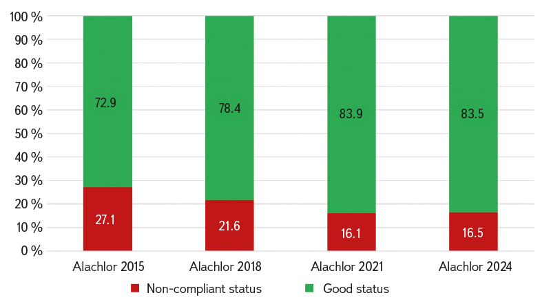
Fig. 17. Proportion of profiles by alachlor metabolite limits in each three-year period
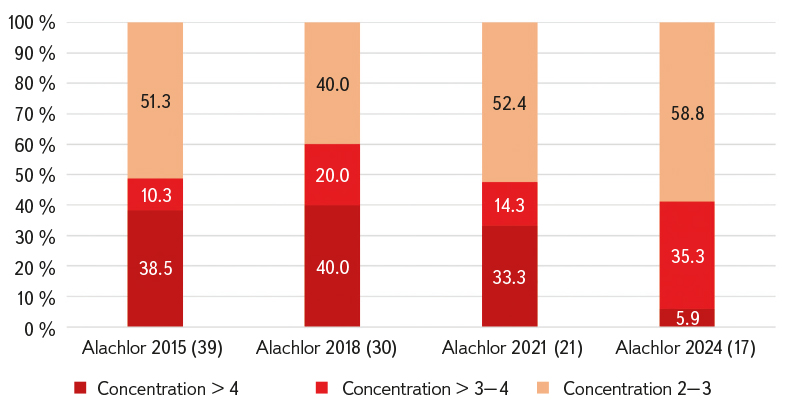
Fig. 18. Proportion of profiles by multiples of the alachlor metabolites concentrations relative to the limit in each three-year period – high concentrations (numbers in the graph in brackets represent the number of profiles)
Adsorbable organically bound halogens (AOX) also showed a pattern similar to that of fluoranthene (Fig. 19). Concentrations declined steadily, the proportion of monitoring sites achieving good status increased by as much as 17.3 percentage points, and in the most recent three-year assessment period no monitoring site had a non-compliance index greater than 2.
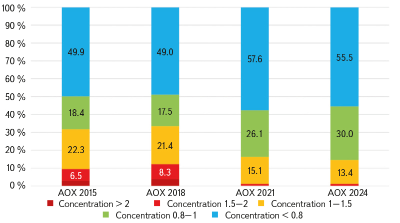
Fig. 19. Proportion of profiles by multiples of the AOX concentrations relative to the limit in each three-year period
The situation is somewhat different for metolachlor and its metabolites (Fig. 20). Although contamination of surface waters is less widespread than for alachlor metabolites (during the 2022–2024 assessment period, only 7.9 % of water bodies in the Czech Republic failed to achieve good status because of metolachlor), the proportion of water bodies failing to achieve good status has remained more or less unchanged. The use of S-metolachlor was also banned in 2024, although this could not yet have been reflected in the assessment period analysed. Nevertheless, metolachlor metabolites can be expected to persist in soils and surface waters for a considerable time.
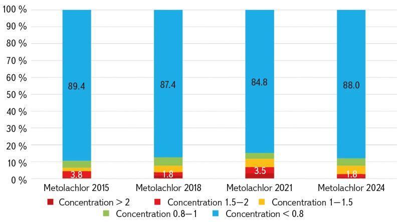
Fig. 20. Proportion of profiles by multiples of metolachlor and its metabolites concentrations relative to the limit in each three-year period
The final specific pollutant assessed was ethylenediaminetetraacetic acid (EDTA). No clear trend in concentrations can be observed, and the difference of 3.5 percentage points is not significant (Fig. 21). However, the highest concentrations, with non-compliance indices exceeding 7, appear to have declined gradually, from 4.9 % of all monitoring sites to 2.5 % (Fig. 22). However, because EDTA has been monitored more extensively only since the 2016–2018 assessment period and the comparison is based on just 203 monitoring sites, this conclusion is not sufficiently supported by the available data.
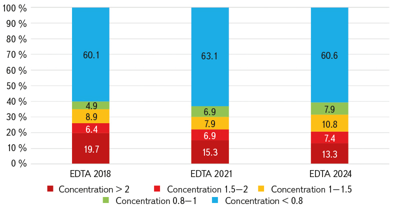
Fig. 21. Proportion of profiles by multiples of the EDTA concentrations relative to the limit in each three-year period
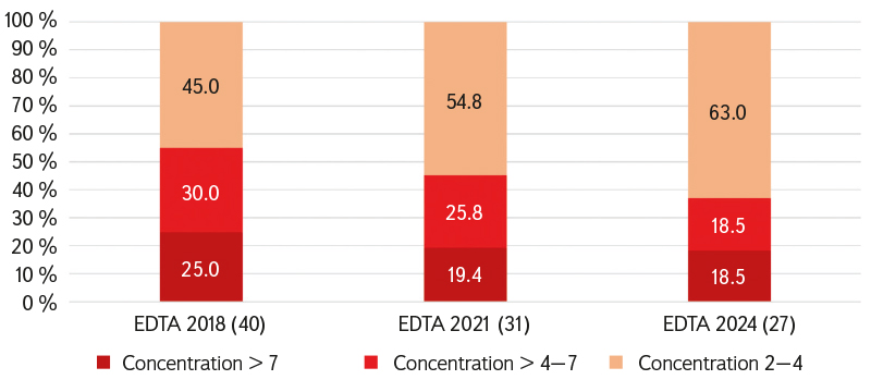
Fig. 22. Proportion of profiles by multiples of the EDTA concentrations relative to the limit in each three-year period – high concentrations (numbers in the graph in brackets represent the number of profiles)
CONCLUSION
To assess trends in the status of surface waters, it is necessary to focus on individual indicators. Three-year assessment periods provide the most appropriate basis for this analysis. They are consistent with the assessment of surface water status and, at the same time, reduce the influence of hydrological extremes, particularly short-term droughts and periods of high flow, on the measured concentrations. Only monitoring sites that were monitored throughout the entire assessment period should be included. The methodology should correspond as closely as possible to the procedures used for classifying chemical and ecological status, using mean values or medians (this approach cannot be applied to maximum or minimum values) and the same good status thresholds (environmental quality standards). Where the assessment methodologies have changed over time, the most recently applicable methodology should be used. This means that status must be recalculated from the primary data. Although it is possible simply to compare the first and the most recent three-year assessment periods, using all five assessment periods provides a much clearer picture of the trends. The methodology is best suited to larger geographical areas. However, once the behaviour of an indicator has been characterised across a large number of water bodies or monitoring sites, differences between individual water bodies or sites can also be investigated. The methodology presented here was developed using data for the whole of the Czech Republic covering the period 2010–2024, i.e. five three-year assessment periods. However, it is not sufficient simply to determine the number of monitoring sites achieving good status. A more suitable approach is to classify the results according to non-compliance index categories (i.e. the ratio of the relevant characteristic value to the good status threshold). For this purpose, non-compliance index categories of 0.8, 1, 1.5 and 2 proved appropriate, with additional categories of 2, 3 and 4, or 2, 4 and 7, where a high proportion of non-compliant results occurred.
The methodology was applied to five general physicochemical indicators (nitrate nitrogen, ammoniacal nitrogen, BOD₅, total phosphorus, and phosphate phosphorus), one priority substance (fluoranthene), and four specific pollutants. All five three-year assessment periods were evaluated for the general physicochemical indicators. For the remaining indicators, data could be used only from the second assessment period onwards because too few monitoring sites were included in the first three-year assessment period, while for EDTA the analysis could begin only with the third assessment period for the same reason.
The analysis showed that nitrate nitrogen and ammoniacal nitrogen concentrations have been declining gradually, while significant improvements were demonstrated for fluoranthene, alachlor metabolites, and AOX. By contrast, concentrations of BOD₅, metolachlor and its metabolites, and EDTA have remained stable, whereas total phosphorus and orthophosphate phosphorus have shown stagnation or even a gradual deterioration. In terms of the effectiveness of the measures implemented, wastewater treatment appears to have been successful in reducing ammoniacal nitrogen concentrations and, probably, industrial wastewater pollution represented by AOX. Diffuse agricultural pollution also appears to have declined, probably owing to a combination of factors, including high fertiliser prices and effective advisory services. Although no measures have been implemented specifically to reduce fluoranthene pollution, concentrations have declined significantly, probably as a result of the gradual closure of some industrial facilities and the continuing reduction in coal mining and combustion. The ban on the use of alachlor in 2006 also contributed to the decline in alachlor metabolites. Nevertheless, water pollution continued to decrease only until the 2019–2021 assessment period and has since levelled off. A similar trend can be expected for metolachlor and its metabolites. However, as their use was not banned until 2024, any improvement is likely to take considerably longer. On the other hand, contamination of surface waters is much less widespread, with only 7.9 % of water bodies failing to achieve good status during the 2022–2024 assessment period.
Although BOD₅ concentrations have remained stable, municipal wastewater treatment can be assumed to be operating effectively, and the remaining elevated concentrations are more likely to originate from other sources. The least progress has been made in reducing total phosphorus and phosphate phosphorus concentrations, probably owing to the high proportion of combined sewer overflows, households not connected to the sewerage system, and soil erosion.
It should be emphasised that the methodology presented here is not intended to replace the assessment of surface water status. The reported values and percentages indicate only how the results change over time; they do not represent the proportions of water bodies achieving or failing to achieve good status, because not all assessment results can be used for comparison. The greater the number of monitoring sites included in the assessment of progress towards achieving good status, the more closely the results reflect the situation for the Czech Republic as a whole. This applies, for example, to nitrate nitrogen and ammoniacal nitrogen, although the status assessment for nitrate nitrogen also includes maximum values in addition to the median, resulting in less favourable status classification results. The assessment of EDTA may be particularly biased because it is based on only 203 monitoring sites.
The Water Framework Directive also prohibits deterioration in status. However, analysis of real-world data confirms that changes in flow conditions can cause concentrations of some indicators to fluctuate, resulting in movement between classification categories. For status assessment, this mainly affects monitoring sites with non-compliance indices in the ranges 0.8–1 and 1–1.5.
As a result, water bodies may move from “good status” to “failing to achieve good status”, even though no genuine deterioration has occurred.
Acknowledgements
This article was prepared as part of research carried out within Project No. SS02030027, Water Systems and Water Management in the Czech Republic under Climate Change, funded by the Technology Agency of the Czech Republic under Subprogramme 3 – Long-term Environmental and Climate Perspectives of Programme SS – Programme for Applied Research, Experimental Development and Innovation in the Environment – Environment for Life. The authors also wish to thank the Vltava River Water Authority, Elbe River Water Authority, Ohře River Water Authority, Morava River Water Authority, and Oder River Water Authority for providing the data used in this study.
The Czech version of this article was peer-reviewed, the English version was translated from the Czech original by Environmental Translation Ltd.
